
DeepStream is a modular, fast library tailor-made for multimedia applications running on Nvidia hardware. In the previous blog, we discussed some DeepStream fundamentals that will get your first video analytics pipeline up and running. The thing is, a naive pipeline implementation almost never lets a model reach its full potential. Often, a pipeline’s “first draft” still has unnecessary format conversions, irrelevant compression and decompression steps, or hardware accelerators that are just not being used.
For example, the GPU can spend loads of time scaling images from a video stream instead of running inference. And while all this is happening, the video/image compositor might be idle when it could be helping with the scaling task. In another situation we’ve seen the pipeline’s inference engine using a slow or buggy NMS implementation, rendering the model’s terrific throughput completely irrelevant.
If you’re a developer who wants to avoid these issues, if you find yourself hitting a wall trying to solve them, or would simply like to identify the exact bottleneck in your DeepStream pipeline, this blog post is for you.
We’ll start with tips that will help you quickly debug dysfunctional pipelines and then delve into how to use NVIDIA’s Nsight Systems to speed up your DeepStream application and bring your model to its full potential.
Free tools for debugging your pipeline
Let’s start with the fact that DeepStream relies entirely on the GStreamer framework and extends it for NVIDIA-specific hardware and use cases. This means you can use DeepStream to easily access basic GStreamer debugging tools.
The first of these useful tools is the GStreamer application’s logger. Most GStreamer plugins provide prints of useful information from interesting points in their code. You can access these prints by simply setting the GST_DEBUG environment variable to match the verbosity you want logged to your stdout/err file descriptors.
The levels range from 0 (no debug information) to 9 (full on memory-dump-level log) with 1 printing all errors, 2 all warnings, and so on. For example, if your application is crashing before generating any output data, there are probably issues with the negotiation stage of the GStreamer pipeline initialization. Rerun the pipeline with GST_DEBUG set to 3 and you’ll see time-stamped prints from stages of the negotiation flow along with the errors encountered.
Below is a toy example of a pipeline that reads in MJPEG format from a camera to an attached screen. You can try removing any elements to spot where the error messages appear in the log:
GST_DEBUG=3 gst-launch-1.0 v4l2src device=/dev/video0 ! image/jpeg,width=640,height=480,framerate=30/1 ! jpegparse ! jpegdec ! autovideosink sync=false
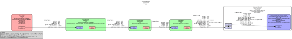
Another simple and nice tool is the pipeline graph exporter. GStreamer lets you get .dot files that illustrate the architecture of your entire pipeline, including dynamically loaded plugins.
Simply set the GST_DEBUG_DUMP_DOT_DIR environment variable and either execute your pipeline through the gst-launch CLI or call GST_DEBUG_BIN_TO_DOT_FILE() (or the corresponding Gst.debug_bin_to_dot_file() Python binding) from within your application’s code.
This gives you a sweet visual representation of the pipeline that will help you understand the flow of data and where performance problems may arise. For example, the diagram below was generated to illustrate the gst-launch command’s pipeline from above:
Nsight Systems for profiling DeepStream pipeline
In many cases, reading through the GStreamer plugin logs or visually inspecting the pipeline’s architecture simply isn’t enough. To truly bring a pipeline to its full potential, you need to correctly utilize the underlying hardware on which it runs.
Maximizing use of the hardware resources is exactly the goal NVIDIA had in mind when they designed NVIDIA Nsight Systems, their system-wide performance analysis tool.
Paired with a low-overhead command-line tool, NVIDIA Nsight Systems provides a timeline of which hardware was active during each part of a workload’s execution. For starters, you can get the correct symbolication or use NVTX, a package for annotating events, code ranges, and resources in your application. Coupled with the correct symbolication and use of NVTX, you can get a call stack of every executed instruction and a clear image of what part of your source code was running at each point in time.
NVIDIA has already annotated most of their DeepStream plugins with NVTX so you don’t have to. Simply generate a report of a typical workload in your pipeline and you’ll see all annotations in the Nsight Systems GUI.
Let’s continue to the next section to understand how this is done.
Installing Nsight Systems
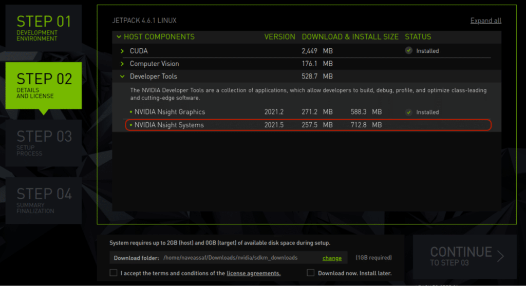
If you’re using a NVIDIA Jetson device, Nsight Systems will be installed as part of the JetPack SDK when you flash your Jetson.
If you’re using a different NVIDIA device, the Nsight Systems CLI should automatically be installed as part of the CUDA ToolKit. In short, you should already have it if you installed the CUDA ToolKit. To check for the installation, simply run the following command on the target device:
sudo nsys --help
On the host machine, where you intend to actually view the generated profiles, install the Nsight Systems image that corresponds to your operating system from the NVIDIA download center.
Enabling Data Collection
Linux blocks the collection of certain scheduling and performance data for security reasons (you can read more about this in the Linux Kernel documentation). To have full visibility into what’s happening on the hardware, you have to disable this behavior. You can do this by altering the value listed in the /proc/sys/kernel/perf_event_paranoid file to be <= 2:
# Temporary modification (does not persist across reboots)
sudo sh -c 'echo 2 >/proc/sys/kernel/perf_event_paranoid'

# Permanent modification
sudo sh -c 'echo kernel.perf_event_paranoid=2 > /etc/sysctl.d/local.conf'

 # Verify (must be <= 2)
sudo cat /proc/sys/kernel/perf_event_paranoid
Generating a Profile Report
The number one rule of profiling is ALWAYS PROFILE A TRULY REPRESENTATIVE WORKLOAD. This means that when generating your profile report you must choose a command that accurately reflects the work your application will be doing.
Simply running your application and interrupting the execution (SIGINT) is likely to create problems in the data collection. It’s better to have your application exit cleanly after a set amount of time or based on some event.
Now that you have a command you intend to profile, run it through the nsys CLI. The -t flag in the example below is critical for selecting the APIs you would like to trace and later view in the Nsight Systems GUI:
# Generic command for generating a report
sudo nsys profile -t [traces to collect] -o [desired path of created report] [command/path to script to profile]

# Example usage for profiling the benchmark of ResNet101 model
ch Resnet101.engine
Analyzing Profiles
Once you have created the report on your host machine, you’re ready to draw conclusions and optimize based on the results. To get started, open the NVIDIA Nsight Systems application and use the File > Open tabs to display your report.
At this point, you may be wondering what you should be looking for. In a typical AI-based video analytics application, the AI model’s inference will be the bottleneck of your pipeline since it’s the most computationally heavy task. Furthermore, your model will likely run on the GPU (unless part of its nodes execute on a DLA) since the GPU is the most powerful hardware in NVIDIA devices.
Basically, if your model is on the GPU and you can reach 100% GPU utilization with the maximum amount of non-inference tasks (like image scaling and reformatting) running on other pieces of hardware (i.e., CPU, VIC, codecs, …), congratulations! This means you’ve reached your pipeline’s theoretical maximum throughput. This is that same throughput you see when benchmarking the model outside of your application.
Below is a profile for a video streaming pipeline with a SOTA object detection model performing the inference. We know that the GPU is being fully utilized because there are no substantial gaps in the CUDA hardware lines of the profile.
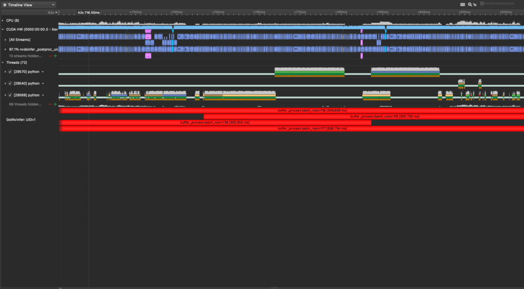
Other than attempting to offload non-inference tasks from the GPU to other hardware, there’s not much room for improvement. We can only improve the detection model itself – so that’s exactly what we did.
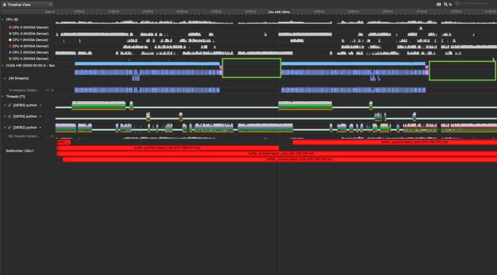
Below is an example of the same exact pipeline, except the GPU is NOT being fully utilized. You can tell by the periodic gaps in the CUDA hardware activity; these are the areas enclosed by green squares. While it’s difficult to observe, this pipeline is actually running faster; even so, the model’s redesign left us much more room for improvement.
The more interesting part comes once we delve deeper into what else is executing during the faster model’s inference:
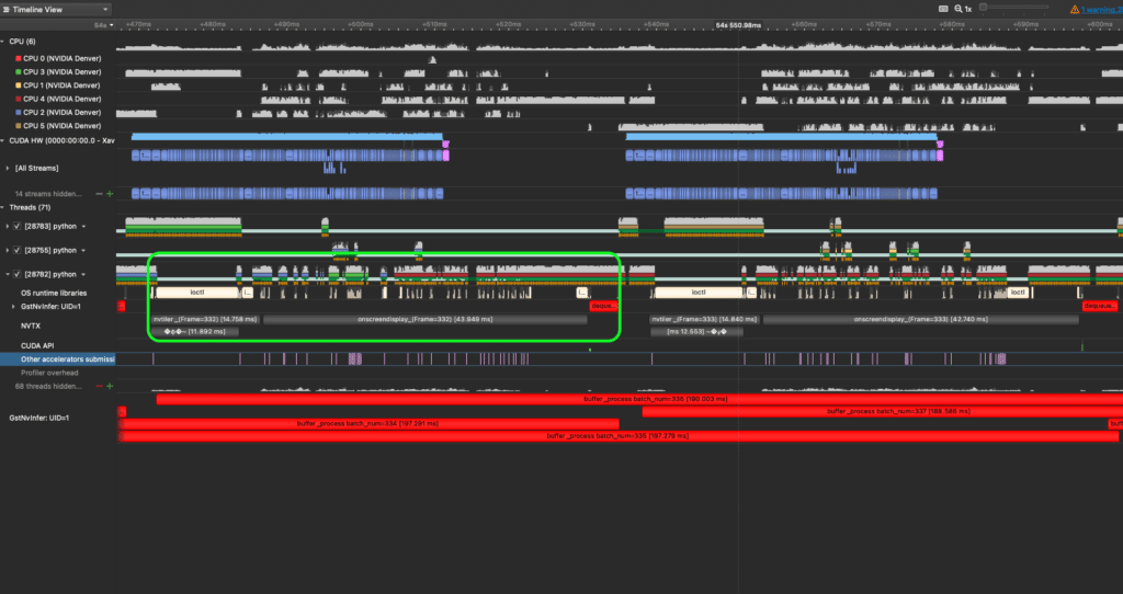
On closer inspection, we can see that the Python thread marked with a green square (28782) periodically performs the following tasks:
- Tiling different video streams into one 2D image (the nvtiler NVTX box)
- Rendering bounding boxes onto this 2D images (the onscreendisplay NVTX box)
- Dequeuing metadata for the next batch before likely syncing with another Python thread (28783).
What’s absurd is that this periodic set of serialized actions together take more time than the model’s entire inference of a batch! This means our second model’s inference latency is faster than the post-processing we are performing.
Just for some context, the faster model is a detection model generated by Deci’s proprietary AutoNAC NAS engine. The slower one is a SOTA YOLOX model, with an mAP 1% lower than Deci’s corresponding model (in both FP16 and INT8 calibrations). Both receive downsampled inputs of 640×640 from input streams of 720p.
How did AutoNAC generate a faster model? AutoNAC, short for automated neural architecture construction, lies at the heart of Deci’s deep learning platform. The platform empowers you to bridge the gap between how a model is currently performing and its full potential when tuned for the correct hardware. This is done using sophisticated Neural Architecture Search algorithms that generate highly accurate and efficient neural networks.
Looking at the profiles from Example 3 , you can see that the AutoNAC-generated model’s latency is so low that to speed up the pipeline you would need to alter the bounding box rendering algorithm, increase the model’s batch size, or try to parallelize the different post processing stages where possible.
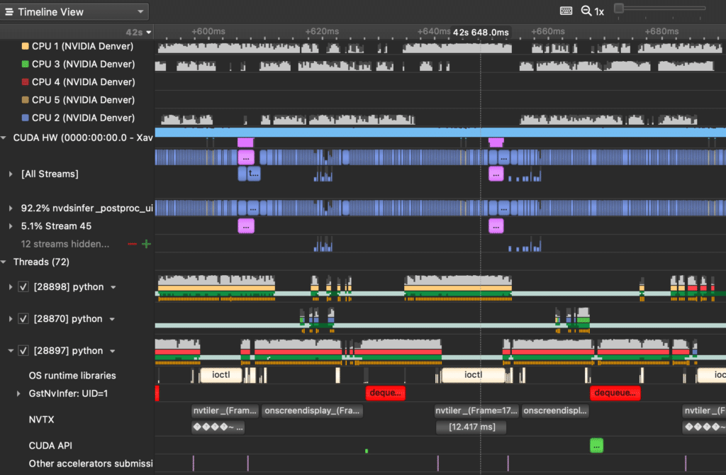
We decided to focus on speeding up the bounding box rendering stage. Ultimately, we were able to reach the desired 100% GPU utilization and theoretical benchmark performance of 192 FPS on a Jetson Xavier NX. This near ideal utilization can be seen in the profile below:
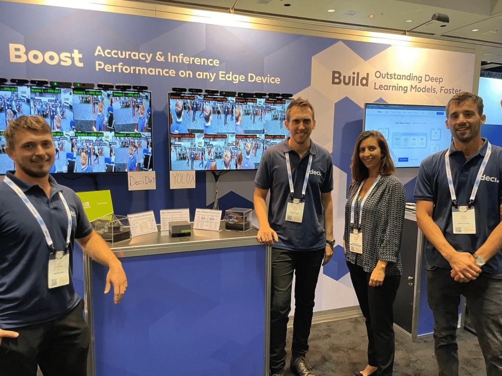
To give a final sense of what can be achieved with a fast model in an efficient DeepStream app, we ran the optimized pipeline discussed above with both the slower SOTA YOLOX model and the AutoNAC generated Deci detection model. Below is an image from the 2022 Embedded Vision Summit where we showcased a side-by-side comparison of the performance of each pipeline.
Tuning your model for maximum performance
This blog walked through a scenario that starts with a basic NVIDIA DeepStream pipeline and showed how you can use profiling to understand where bottlenecks exist. We also saw how you can speed up your application and bring your model to its full potential. Using Deci’s AutoNAC, we were able to build a new custom model for the target hardware and reach that performance sweet spot.
If you found this example interesting, stay tuned for future blog posts on DeepStream profiling case studies, where we share more examples on how profiling can help models reach their full potential.