
TensorRT is a model inference framework by NVIDIA that runs on NVIDIA GPUs. If you are a data scientist or a deep learning engineer, no matter what computer vision tasks you are working with, you have almost certainly encountered TensorRT, which can deliver approximately 4 to 5 times faster inference than the baseline model. While you may be familiar with TensorRT, it is also important to understand the mechanics behind it.
In the first part of this blog, we will provide a general overview of what a model inferencer does, what a deep learning model is composed of, and how to perform inference on it. In the second section, we will dive into the internals of the model inferencer, TensorRT, including the TensorRT compiler and runtime.
In order to understand the internals of TensorRT, you must first understand what a model inferencer does, and to do that you need to understand what we are performing inference on – a deep learning model.
Let’s start with understanding what a deep learning model is and how we represent it.
What is a Deep Learning Model Composed of?
A deep learning model is represented by a computational graph. This graph is made up of inputs that change during operations, parameters or weights, and kernels. In order to understand the rest of this blog it is important that you understand these terms:
- Inputs – Data that is fed to the model, such as images of dogs for an image classification model.
- Architecture – The architecture of the model is the graph itself.
- Weights – The weights are parameters of the model and they are tweaked when training the model. They become fixed parts of the graph when the model is ready for inference.
- Kernels – A kernel refers to a piece of code that implements the “operation” of the layer (a deep neural network is made up of many layers), for example, convolution, relu, etc. There can be numerous implementations for these “high-level” or logical operations in the graph.
The kernel is responsible for implementing a specific algorithm and the inferencer determines which kernel is best. The kernel is considered within the context of the entire model. A kernel is often highly optimized for performance for specific parameters or specific hardware.
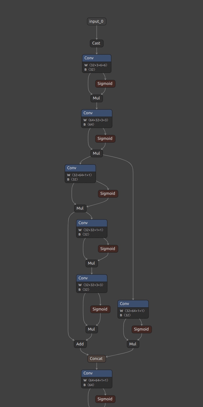
The graph above shows the flow of data from the input (image or video) to the outputs of the model (detections). The “nodes” represent different operations being performed as well as their parameters. These parameters are learned when training the model, but during inference, you can treat them as constant parts of the model. The only thing that changes between executions is the input.
These are local operations, and this graph doesn’t specify how to run the model – that is the task of the compiler.
Now that we’ve gone over what a deep learning model is composed of and how we represent it, let’s understand what it means to perform inference on one.
What is a Deep Learning Model Inferencer?
Deep learning model inference is the process of using a trained deep neural network (DNN) to make predictions about new data. A deep neural network is an algorithm composed of inputs (new data) and outputs. To perform deep learning inference, you feed new data (such as images) into the network which the DNN classifies.
A fully trained DNN should make accurate predictions as to what an image represents. Once a DNN has been fully trained it can be copied to other devices. This typically occurs after a deep neural network has already been simplified and modified to reduce computing power, energy, and memory footprint.
Fully trained deep neural networks can be very large, possessing hundreds of layers of artificial neurons and billions of weights connecting them. The larger the deep neural network, the more compute power, storage space, and energy it will need to run, which will likely also increase latency.
Models contain many different parameters and are “trained” or tweaked to perform as accurately as possible. During inference, these weights are fixed, and your only job is to run the model as quickly as possible.
One solution to the barriers of training and modifying a deep neural network is an inferencer such as TensorRT. TensorRT can run on edge devices, which is often preferable to the cloud. Performing inference analysis on edge devices eliminates many challenges associated with the cloud such as costs, compute power, and latency.
Now that we have a good overview of how a model inferencer works, let’s delve into the internals of TensorRT.
How does TensorRT work?
The TensorRT inference engine makes decisions based on a knowledge base or on algorithms learned from a deep learning AI system. The inference engine is the processing component in contrast to the fact-gathering or learning side of the system.
Inference engines are responsible for the two cornerstones of runtime optimization: compilation and runtime.
- Compilation – The process of deciding which layers and kernels to run for each of the “logical blocks” in the graph, etc. We will go into greater detail on this subject in a later section.
- Runtime – The process of running the graph with the goal of executing the model as efficiently as possible.
The benefit of separating the inferencer into two phases is that all runtime decisions can be made during the compilation phase.
Let’s dive into how the compiler works in greater detail.
The TensorRT Compiler
Compilers compress a DNN and then streamline its operation so it runs faster and consumes less memory. This allows developers to cope with massive computing demand, making graph compilers essential for enabling inference for many applications.
Model compilation is a technique that makes the model faster almost for free and without necessarily impacting accuracy. The compiler modifies the model for the given hardware, while memory allocation and computation are done more efficiently. This is done by evaluating and fixing the computation graph of a given model, from which the compiler then generates an optimized inference code.
Remember in the previous section when we discussed computational graphs? Well, the complexity of the graph grows linearly with the network size. This is where graph compilers come into play.
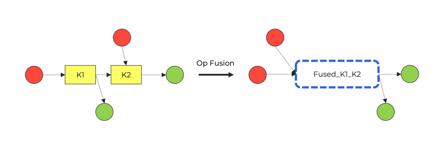
Their goal is to optimize the generated graphs for high-performance inference on target hardware. Graph compilers often combine – or ‘fuse’ – operations where possible and eliminate unnecessary operations. They combine some operations together using a kernel that implements the combined operation (e.g. conv + activations).
The TensorRT compiler uses a series of strategies to measure and test every possible implementation for each operation. It then selects the best kernel based on these tests. This is no simple process as not every kernel or implementation will work well on any hardware.
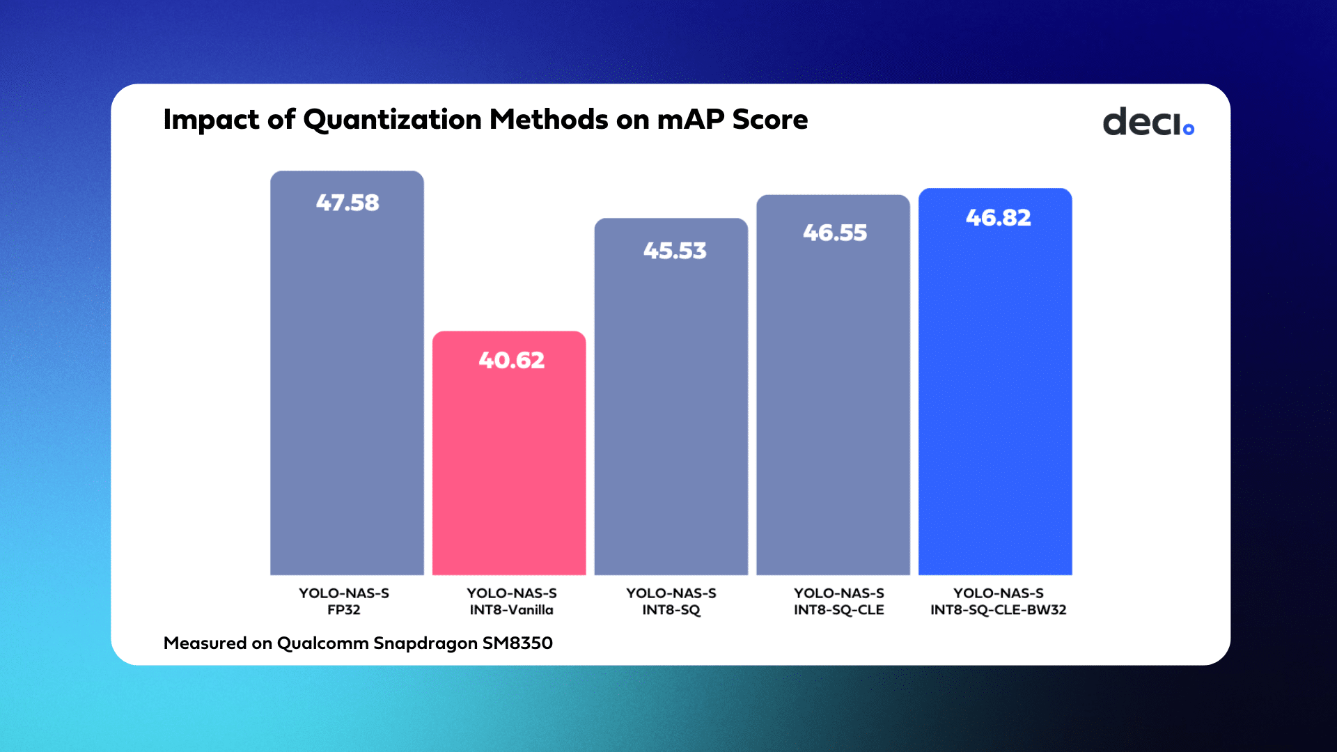
TensorRT may opt to simplify or modify the graph. This can be done by means of fusions or combining some operations together using a kernel that implements the combined operation. It may also do mixed quantization for different layers in order to utilize more of the hardware. Mixed quantization can run different layers of the graph at various precisions to maximize performance without compromising accuracy.
A Production-Aware Process
There are numerous considerations that must be taken into account when selecting an implementation. This is known as a “hardware-aware” process. Variables that influence model efficiency are considered at the beginning of the development process rather than at the end.
Many developers do not do this, waiting until their model is slated to go to production before taking these considerations into account. By then it is often too late and their model may not work on the intended hardware.
Some important considerations include:
- Type of hardware
- Memory footprint
- Input and output shape
- Weight shapes
- Weight sparsity
- Level of quantization
While it may seem like a daunting task to consider all of the above variables, there is an easy solution. The TensorRT inferencer runs a large number of experiments, measures them, and selects the best one based on the model. This solution takes into account all of the conditions outlined in this section.
The TensorRT Runtime
Now that you understand the compiler phase, let’s go over the second component of TensorRT: the “engine” or runtime. The TensorRT engine is represented by the same graph we discussed earlier. Each “layer” in the engine already contains the kernel that will run the operation efficiently on the target hardware. The TensorRT runtime can now load the engine to the device and run it efficiently.
TensorRT’s runtime component is responsible for managing the host-device memory copies and model executions, and sometimes multiple contexts of executions.
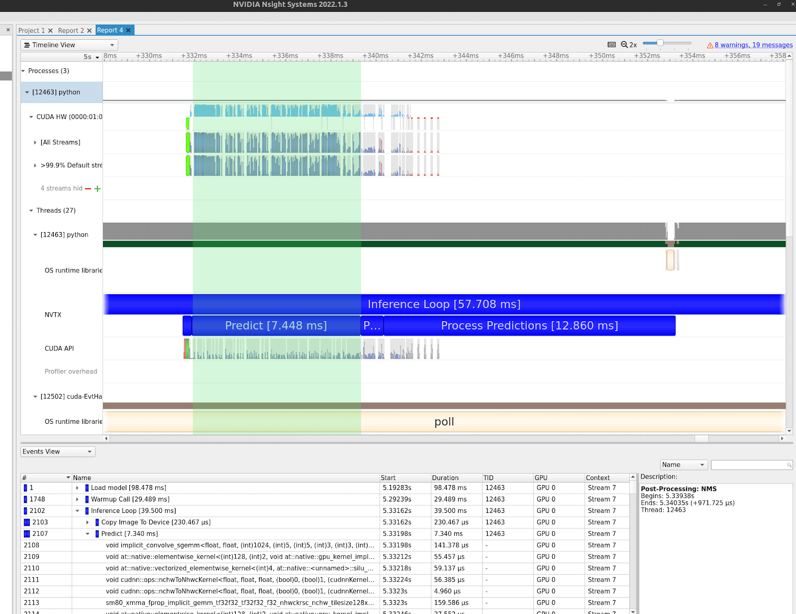
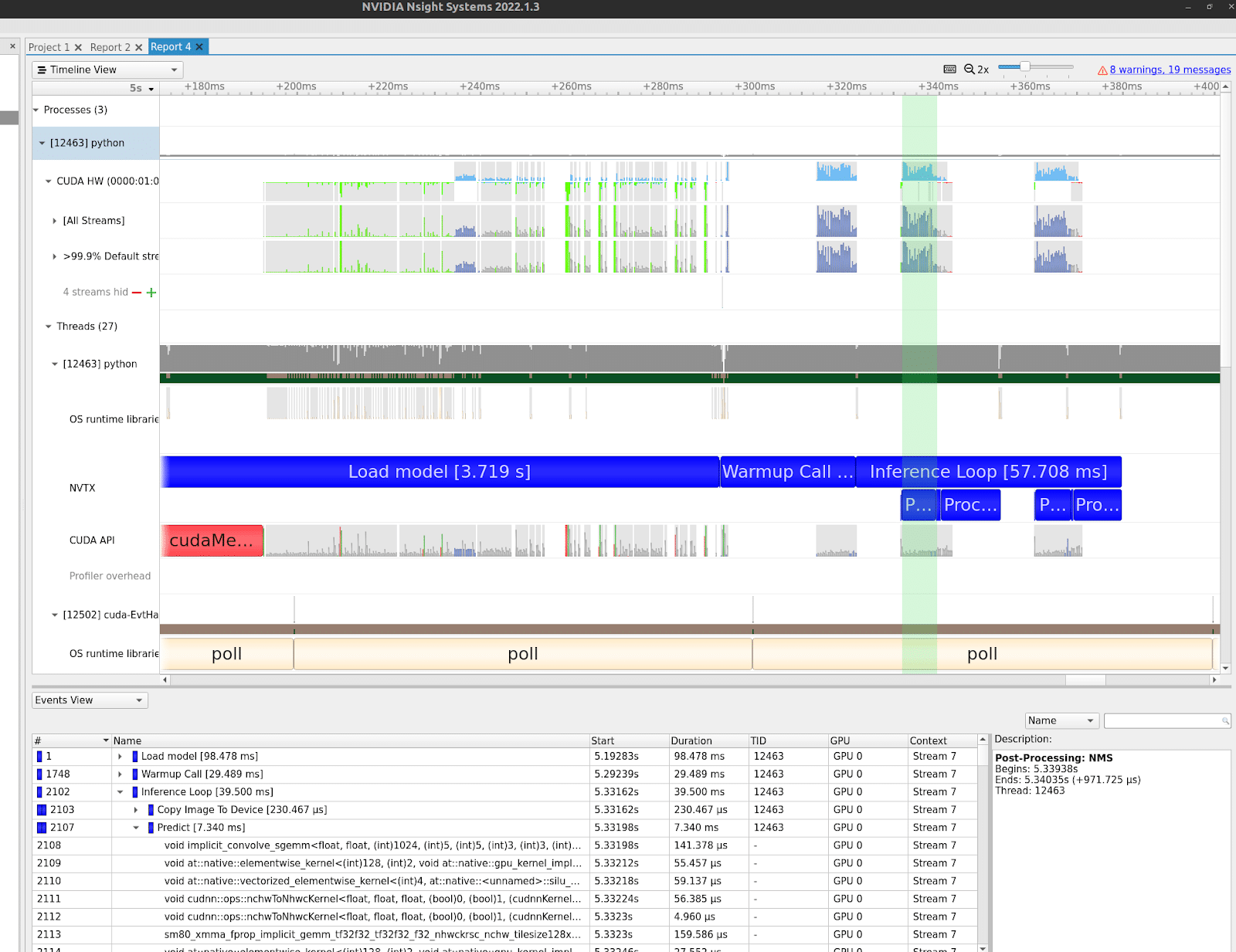
These images show a performance profile of YOLOv5’s detect.py detection example. This is a Python example demonstrating end-to-end detection using a YOLOv5 model. This would be the “naive” initial example to start developing a detection production application.
The images show how different system resources are used over time. The vertical axes represent different system resources, with the NVIDIA GPU at the top, followed by CPU threads, system calls, etc. The highlighted green section in each image is a single forward pass of the model. This is what the TensorRT compiler and runtime will ultimately optimize.
As depicted in these images, different sections of the program require different hardware resources. The model forward pass requires a lot of GPU compute time and some GPU memory IO time. Post-processing NMS algorithms and the actual prediction processing require some GPU resources and a significant CPU overhead. This is also true regarding data acquisition, which is mostly CPU and network, disk, or memory bound.
It is important to note that all of these hardware resources can function in parallel. While the GPU is computing, its memory controller copies data to and from the device. The CPU can handle past and future predictions while the GPU processes current ones.
TensorRT’s runtime component is responsible for utilizing these resources efficiently for the duration of the kernel execution. The runtime component chooses when to run various parts of the graph. This includes many different moving parts.
While code should be written in a way that takes advantage of different hardware resources, as depicted in the previous image, often the model runs serially, only beginning one step after completing the previous one. If this program took advantage of concurrency features like async methods or multi-threading, it would look very different.
For example, let’s assume that GPU compute is the most time-consuming step of the process. A fully concurrent implementation would utilize the GPU 100% of the time, with all prediction sections running on the GPU. While the GPU analyzes one batch of data, the CPU acquires the next batch and processes the previous one.
TensorRT runtime can define multiple execution contexts for the same model. This allows multiple executions to be queued at once – without the model inputs and outputs being overwritten by the different contexts.
Further Considerations: Beyond TensorRT
In this blog, we discussed what a model inferencer does, and specifically how TensorRT optimizes model prediction on a GPU. We’ve outlined the internal components and processes of the TensorRT compiler, as well as its function during runtime.
However, there are many other components, and once you optimize one bottleneck, something else emerges as a problem. If you want to maximize performance, TensorRT is only one step. There is far more to do afterward.
Other considerations include:
- Where to process your data
- How to acquire data
- How many batches to execute concurrently
- What size should the batches be
Compiling the model and using the appropriate runtime for your hardware is just the first step in the optimization process. To get the best performance from your prediction pipeline you must understand how the whole system works.
Remember to consider the entire prediction pipeline when developing your program – not just the engine inference. Fully utilize all of your hardware resources to get the most out of your hardware and maximize your model performance.
Check out Deci’s hardware-aware deep learning platform to get the most out of your models. You can benchmark your models and compare accuracy, performance, and other metrics across various hardware. Start benchmarking your models and get the best model performance now.