As deep learning models have grown in their complexity and applications, they’ve also grown large and cumbersome. This has direct implications on both cloud and edge deployments.
This article discusses model quantization in detail. It goes over its benefits and compares post-training quantization (PTQ) to quantization-aware training (QAT).
Large models running on cloud environments have huge compute demand resulting in high cloud cost for developers, posing a major barrier to profitability and scalability. For edge deployments, edge devices are resource-constrained and therefore are limited in their ability to support large and complex models.
Whether the model is deployed on the cloud or at the edge, AI developers are often confronted with the challenge of reducing their model size without compromising model accuracy. Quantization is a common technique used to reduce the model size, though it can sometimes result in reduced accuracy.
Quantization-aware training is a method that allows practitioners to apply quantization techniques without sacrificing accuracy. It is done in the model training process rather than after the fact. The model size can typically be reduced by two to four times, and sometimes even more.


There are different representations of floating-point numbers. Common ones used in deep learning are 32-bit and 16-bit floats (FP32 and FP16 respectively). For acceleration of deep learning and high performance, there are hardware-specific floating point formats, like NVIDIA’s TensorFloat (TF32), Google’s BrainFloat (bfloat16), and AMD’s FP24. There are smaller formats, which are colloquially called minifloats. These formats, like FP8, are usually used in microcontrollers for embedded devices. Their support was announced in the new generation of NVIDIA’s GPUs like H100.
Double precision formats like float64 are rarely used in the context of deep learning because of the large memory overhead and no benefit for deep neural networks, so we will not cover them here. However, their usage can be beneficial for statistical modeling, where single precision is not enough.
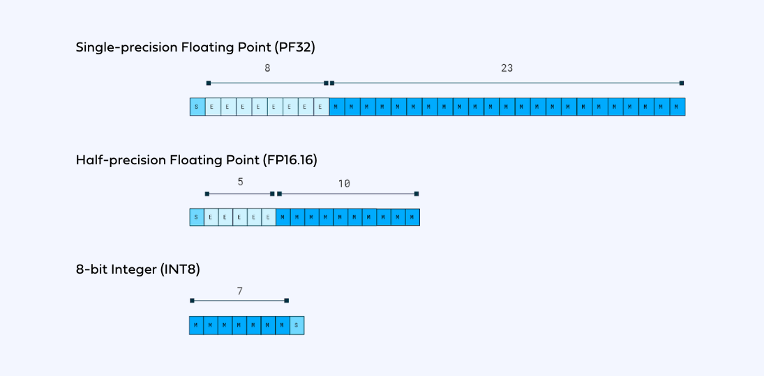
Quantization is a model size reduction technique that converts model weights from high-precision floating-point representation to low-precision floating-point (FP) or integer (INT) representations, such as 16-bit or 8-bit. By converting the weights of a model from high-precision floating-point representation to lower-precision, the model size and inference speed can improve by a significant factor without sacrificing too much accuracy. Additionally, quantization will improve the performance of a model by reducing memory bandwidth requirements and increasing cache utilization.
In the context of quantization of deep neural networks, INT8 representation is colloquially referred to as “quantized”. However, other formats are used, for example, UINT8, which is the unsigned version, or INT16, which can be used on x86 processors.
Different models require different approaches to quantization, and successful quantization often requires prior knowledge and extensive finetuning. In addition, quantization can introduce new challenges and trade-offs between accuracy and model size, particularly when using low-precision integer formats such as INT8.
Quantization can also introduce some challenges, particularly when using low-precision integer formats such as INT8. One major challenge is the limited dynamic range of these formats, which can lead to a loss of accuracy when converting from higher-precision floating-point representations.
While FP16 can be used instead of FP32 with only a small loss in accuracy of the representation in the context of deep neural networks inference, the smaller dynamic range formats like INT8 pose a challenge. During quantization, we have to squeeze a very high dynamic range of FP32 into only 255 values of INT8, or even into 15 values of INT4!
To mitigate this challenge, various techniques have been developed for quantizing models, such as per-channel or per-layer scaling, which adjust the scale and zero-point values of the weight and activation tensors to better fit the quantized format. Other techniques, such as quantization-aware training, can also help to prepare a model for quantization by simulating the quantization process during training.
This squeeze (estimating the range) is done with a process called calibration.
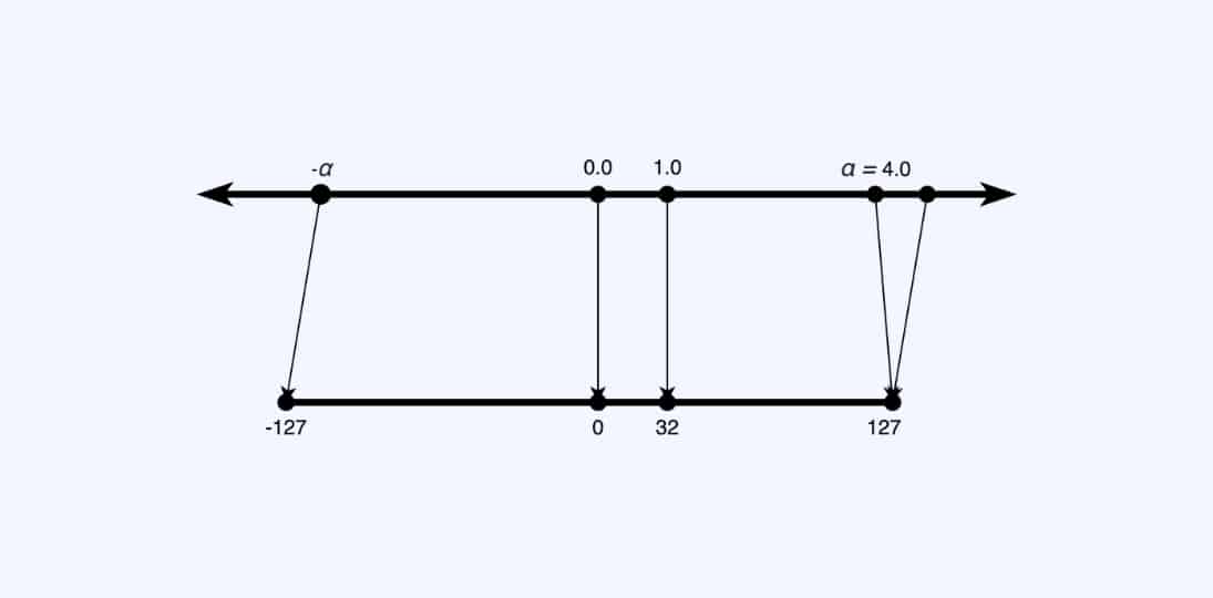
The input range is x ∈ [-α, α], and the maximum α value (amax) is calibrated to maximize precision. Once α is calibrated, the mapping is performed by multiplying/dividing by a scale factor s. This approach is called scale quantization.
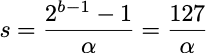
Everything in the dynamic range outside α-interval will be clipped, and everything inside it will be rounded to the nearest integer. We have to be careful selecting these ranges – large alphas will “cover” more values, however, result in coarse quantization and a high quantization error nonetheless, so the selection of these ranges is usually a tradeoff between clipping error and rounding error.
The calibration process can be performed using different methods, depending on the requirements of the model and the use case.
Most commonly supported are percentile, max, and entropy methods that are supported by the majority of frameworks.
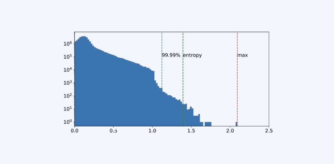
Here we can see a Histogram of input activations to one of the layers in ResNet50 and calibrated ranges (alphas) using different methods (image source).
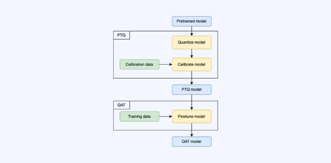
Post-training quantization (PTQ) is a quantization technique where the model is quantized after it has been trained.
Quantization-aware training (QAT) is a fine-tuning of the PTQ model, where the model is further trained with quantization in mind. The quantization process (scaling, clipping, and rounding) is incorporated into the training process, allowing the model to be trained to retain its accuracy even after quantization, leading to benefits during deployment (lower latency, smaller model size, lower memory footprint).
There’s no need for calibration after the QAT process because the model is calibrated in the training process. This training optimizes model weights to improve model performance on downstream tasks by emulating inference-time quantization. It uses “fake” quantization modules, called Q/DQ (quantize then de-quantize), during training to imitate the behavior of the testing or inference phase. The weights of DNNs, for example, are rounded or clamped to 16-bit floating point or 8-bit integer representations during training.
The neural network’s forward and backward pass uses low-precision weights. The loss function adjusts the model for low-precision calculation errors. As a result, the quantized model allows higher accuracy during real-world inference as the model was made aware of quantization during training.
As seen in the figure (image source), QAT incorporates quantization during the training process, which means that the model is optimized to perform well in a quantized environment from the get-go. In contrast, PTQ applies quantization after training, which can result in a loss of accuracy due to the mismatch between the original model and the quantized model. Moreover, QAT allows for finer-grained control over the quantization process, as different layers or even individual weights and activations can be quantized differently depending on their sensitivity to quantization errors. This results in better accuracy retention.
So far, we’ve covered the various levels of quantization to consider, as well as some methodologies for when it should be applied. However, when trying to quantize your models, there is another factor to consider which is – what type of quantization will yield the optimal results for your needs. In this section, we’re going to compare three types of quantization.
In naive quantization, all operators are quantized to INT8 precision, and are calibrated using the same method.
Keep in mind that some architecture layers are sensitive and therefore, the accuracy will drop dramatically. For example, in single-stage detection models, like YOLO, the last layers for classification and bounding-box regression are the most sensitive, so it’s a common practice to exclude them.
In addition, some sequences of operators are not friendly for INT8 – latency will not improve (and even get worse!). Inference frameworks fuse sequences of operators into a single one (like Conv-BN-ReLU), so the execution is way faster on the supported hardware. This will be impossible if some of these operators are in different data types.
Also, some operators can not be fused in INT8, only in FP16, like GroupConv-BN-Swish in NVIDIA’s TensorRT 8.4, which heavily depends on the hardware, inference framework, and its version. It will be better to leave them in FP16 both for latency and accuracy.
While being easy to implement, naive quantization often results in a significant drop in model accuracy compared to the original floating-point model. This is because the same quantization method is applied to all operators, regardless of their sensitivity to quantization. In contrast, using more sophisticated quantization methods, such as hybrid or selective quantization gives better results in terms of latency and accuracy.
In hybrid quantization, some operators are quantized to INT8 precision, and some are left in mode representative data type like FP16 or FP32.
In order to do it, you have to have prior knowledge of the neural network structure and its quantization-sensitive layers, or you need to perform a sensitivity analysis: exclude layers one-by-one and watch the change in latency/accuracy.
Some blocks need special structure for successful conversion with inference frameworks like NVIDIA TensorRT. While its compiler can fuse Conv-BN-ReLU, it requires special consideration with Conv-BN-Add sequence, adding one more quantizer to the other input of Add operation. That is especially prominent, with residual connections that are in the majority of modern CNNs, especially ResNet. The whole sequence of operators will not be quantized if there is a non-quantized addition somewhere, and the latency will be worse.

In selective quantization, some operators are quantized to INT8 precision, with different calibration methods and different granularity (per channel or per tensor), residuals are quantized to INT8, as well as sensitive and non-friendly layers remain in FP16 precision. Additionally, with selective quantization, we can change whole parts of the model to better suit quantization. This type gives users the most flexibility in the selection of quantization parameters for different types of the network to maximize accuracy and minimize latency simultaneously.
For example, models, like RepVGG, have vastly different distributions in their branches, so it is usually better to quantize different layers with different calibrations in mind. Some will be better with max calibration, and others will have outliers and are better with percentile to remove them – so we can use different calibrators for different layers. Activation distributions are different and different calibrators are needed for weights and activations.
Why use selective quantization?
After learning about the various factors to address when quantizing your models. Now let’s deep dive into some essential best practices to follow when applying quantization to deep learning models to achieve the desired level of accuracy and performance.
These practices include carefully selecting the appropriate quantization method, identifying sensitive layers, and fine-tuning your models using quantization-aware training. Additionally, there are several hyperparameters that should be carefully tuned to ensure that your quantized model performs optimally.
In the following section, we’ll discuss some rules of thumb for hyperparameter values for your quantization procedure, which are an aggregation of NVIDIA’s best practices together with our own experience.
Use per-channel granularity for weights and per-tensor for activations
Weight tensors have vastly different distributions of values per channel, and quantizing it with a single scale factor may result in significant accuracy loss. By using per-channel granularity for weights, the distribution of values within each channel can be better preserved during quantization. Also, inference frameworks will fold per-channel scales into kernels, so there will be no computational overhead during inference. As neural networks are usually trained with weight decay, weight distributions within channels are usually compact, so it is beneficial to capture all the dynamic ranges and use Max calibrators for weights.
On the other hand, activations are typically more consistent across channels and usually contain outliers from different input data points. Using a single scale factor for all channels in an activation tensor in a given layer can help to minimize the impact of the outliers, especially by using histogram-based methods. Also, as these scales cannot be folded into a kernel, using only a single scalar per tensor reduces computational overhead.
Quantize residual connections separately by replacing blocks
Residual connections are an important component of many deep learning models like ResNet, as they help to mitigate the vanishing gradient problem that can occur during training. However, when it comes to quantization, residual connections can pose a challenge. The reason for this is that inference frameworks like NVIDIA’s TensorRT require a single data type for all operations in order to fuse them into a single kernel. If the residual connections use a different data type than the other layers in the model, it can prevent these layers from being fused and can lead to decreased performance.
The best way to address this issue is to quantize residual connections separately from the other layers in the model. This involves replacing each residual connection with a quantized block that includes a quantized version of the identity mapping that is added to the input of the quantized block. By doing this, the residual connections can be quantized to the same data type as the other layers, allowing them to be fused together and improving performance.
Identify sensitive layers and skip them from quantization
While many layers can be effectively quantized without sacrificing too much accuracy, there are certain types of layers that can pose a challenge for quantization. These include layers that represent a bottleneck in the model, as well as layers that perform operations that require higher precision in order to maintain accuracy.
One common example of a layer that is sensitive to quantization, is the last layer of a detection model that performs bounding box coordinate regression. This layer typically requires high precision in order to accurately predict the coordinates of object bounding boxes, and quantizing it can result in a significant loss of accuracy. As a result, it’s often recommended to skip this layer from quantization.
In order to determine which layers in a particular model are likely to be sensitive to quantization and need to be skipped, it’s often necessary to perform a sensitivity analysis. This involves quantizing the model and evaluating its accuracy on a validation set to identify which layers are most impacted by quantization. One common approach to sensitivity analysis is to use a technique known as layer-wise analysis, which involves quantizing the model layer-by-layer and evaluating its accuracy at each step. This can help to identify which layers are most sensitive to quantization and need to be skipped.

Start with the best-performing calibrated PTQ model
Rather than starting the quantization-aware training process with an untrained or randomly initialized model, starting with a PTQ model that has already been calibrated can provide a better starting point for the QAT process. This is especially important for low bit-width quantization, where training from scratch can be challenging, and starting with a well-performing PTQ model can help to ensure faster convergence and better overall performance.
Fine-tune for around 10% of the original training schedule
Quantization-aware training should not take as long as the original training process, as the model is already relatively well-trained and only needs to adjust to the lower precision. In general, fine-tuning for around 10% of the original training schedule is a good rule of thumb.
Use cosine annealing LR schedule starting at 1% of the initial training LR
Using a cosine annealing learning rate schedule can help to improve convergence and ensure that the model continues to learn throughout the fine-tuning process. Starting the schedule at a lower learning rate (e.g. 1% of the initial training LR) can also help to ensure that the model adjusts to the lower precision more gradually and with more stability. Using learning rate warmup with cosine annealing improves stability in the early stage of QAT.
Use SGD optimizer with momentum instead of ADAM or RMSProp
While ADAM and RMSProp are popular optimization algorithms for deep learning, they may not be as well-suited for quantization-aware fine-tuning. These methods rescale gradients per-parameter, which can disrupt sensitive quantization-aware training. Using SGD with momentum can help to ensure that the fine-tuning process is stable and that the model is able to adjust to the lower precision in a more controlled manner.
As you can see, there’s a lot to think of when quantizing your models. To save you lots of time and headache we implemented these rules and more as parameters in SuperGradients, Deci’s open source computer vision training library.
SuperGradients is Deci’s open source “all-in-one” deep learning training library for PyTorch-based computer vision models. It supports the most common computer vision tasks, including object detection, image classification, and semantic segmentation with just one training script.
You can easily get various architectures and train them from scratch or use our pre-trained models which will save you the time of searching for the right model on various places and papers, the overhead of integration and implementation, and many training iterations.
With SuperGradients, you can also save time by using classes, functions, and methods that were already tested and used by many others (like when you use PyTorch or NumPy, and not implement yourself). You can use our recipes to easily reproduce our SoTA reported results on your machine and save time on hyperparameter tuning while getting the highest scores.
Last but not least – all of the pre-trained models in the repo were tested and validated for the ability to compile into production frameworks and include all the documentation, code examples, notebooks, and user guides that you need to do it yourself – no other repo takes production readiness into consideration.
The post-training quantization and calibration procedure in SuperGradients looks like this:
					model = models.get(model_name="resnet18", pretrained_weights="imagenet")

q_util = SelectiveQuantizer(
    default_quant_modules_calibrator_weights="max",
    default_quant_modules_calibrator_inputs="histogram",
    default_per_channel_quant_weights=True,
    default_learn_amax=False,
    verbose=True,
)
q_util.quantize_module(model)  # model now has Q/DQ layers in it!


calibrator = QuantizationCalibrator()
calibration_dataloader = dataloaders.imagenet_val()
calibrator.calibrate_model(
    model,
    method="percentile",
    calib_data_loader=calib_dataloader,
    num_calib_batches=16,
    percentile=99.99,
) # PTQ done! Model is now calibrated!
Applying selective quantization is also easy as pie:
					# skip some layers from quantization
q_util.register_skip_quantization(layer_names={"layer4.0.conv1", "linear"})


# replace BasicBlock with QuantBasicBlock for layers 1-4
q_util.register_quantization_mapping(layer_names={"layer1", "layer2", "layer3", "layer4"}, quantized_target_class=QuantBasicBlock)

q_util.quantize_module(model)  # model is now quantized
calibrator.calibrate_model(
    model,
    method="percentile",
    calib_data_loader=calib_dataloader,
    num_calib_batches=16,
    percentile=99.99,
)
# PTQ done! Model is now quantized and calibrated!
To launch quantization-aware training with best-practice recipe modifications, you can use the YAML file:
					ptq_only: False
selective_quantizer_params:
  calibrator_w: "max"
  calibrator_i: "histogram"
  per_channel: True
  learn_amax: False
  skip_modules:

calib_params:
  histogram_calib_method: "percentile"
  percentile: 99.99
  num_calib_batches: 16
  verbose: False
If you want to use our rules of thumb to modify your existing training recipe parameters for quantization-aware training, you need to use QATRecipeModificationCallback. To do it, add the following config to your recipe:
					pre_launch_callbacks_list:
  - QATRecipeModificationCallback:
      batch_size_divisor: 2
      max_epochs_divisor: 10
      lr_decay_factor: 0.01
      warmup_epochs_divisor: 10
      cosine_final_lr_ratio: 0.01
      disable_phase_callbacks: True
Default parameters of this callback are representing the rules of thumb to perform successful quantization-aware training from an existing training recipe.
Now that you are done, the last step for post-training quantization and quantization-aware training is compiling the model with NVIDIA TensorRT (8.4+) in order to transform the model with Q/DQ into 8-bit hybrid representation.
In order to do that, Deci users can easily use the Deci platform API and optimize the model to INT8 quantization with a click of a button. This is a seamless step that will yield a .trt/.pkl engine file that is optimized, quantized, and ready for deployment.
Have a Deci account but didn’t get your API token? Enter the Deci platform and retrieve your API_Key.
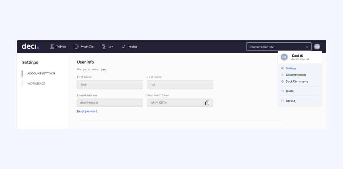
Create a client of Deci Platform and login.
					from deci_lab_client.client import DeciPlatformClient
from pytorch_quantization import nn as quant_nn

client = DeciPlatformClient()

client.login(<API_KEY>)
Compile and optimize the nn.module using Deci platform API via add_and_optimize_pytorch_model function.
					# The `model` variable should contain an instance of `nn.Module`
quant_nn.TensorQuantizer.use_fb_fake_quant = True

client.add_and_optimize_pytorch_model(model, name="resnet18_int8", dl_task="Classification", description=None, hardware_types=["T4"], accuracy=None, input_dimensions=[3, 224, 224], channel_first=True, primary_batch_size=1, quantization_level="INT8", raw_format=False)

quant_nn.TensorQuantizer.use_fb_fake_quant = False
Now you can download the production ready model file from the Deci platform (using the API or the UI) and deploy it using Infery (Deci’s inference engine).
In conclusion, we have gone over how using INT8 quantization can boost inference performance, how you should be aware of the possibility of accuracy reduction and why it happens, and how to leverage SuperGradients’ QAT and selective quantization capabilities in order to preserve the model’s accuracy while achieving INT8 runtime performance.
It’s important to understand that while INT8 quantization can significantly boost efficiency, there’s a ceiling to the performance improvements it can alone provide. To truly maximize performance, it’s essential to pair quantization with other inference acceleration techniques, from optimal model architecture selection to inference pipeline optimization.
To learn more about these inference acceleration techniques, download our comprehensive guide.
Share

Deci is ISO 27001
Certified
					from transformers import AutoFeatureExtractor, AutoModelForImageClassification

extractor = AutoFeatureExtractor.from_pretrained("microsoft/resnet-50")

model = AutoModelForImageClassification.from_pretrained("microsoft/resnet-50")