
At the beginning of the deep learning era, our main goal was to reach new levels of accuracy. Indeed, the early works of deep learning show remarkable results on various tasks and datasets. In recent years, however, the focus has moved to maximizing efficiency. Nowadays, the deep learning community is seeking more accurate models with improved inference efficiency. The notion of efficiency in deep learning inference depends on the context. It might refer to energy consumption, memory efficiency, or run-time efficiency — which is the focus of this post.
Analyses of efficient models that have begun to emerge in recent years often assume that floating-point operations (FLOPs) can serve as an accurate proxy for any kind of efficiency, including run-time. This assumption is clearly wrong in the context of serial vs. parallel computation; when N workers are available it is 1/N faster to dig a moat (a perfectly parallelizable task) than to dig a well (an inherently serial task). Analogously, due to the high parallelization capabilities of the GPU, parallelizable operations will run faster than non-parallelizable operations. But parallelization considerations aren’t everything, and in this post let’s look at a non-trivial example showing that FLOPS are not sufficient for measuring run-time in the context of GPU computation.
In our numerical example, we use the standard CuPy and PyTorch libraries to perform matrix multiplications on a GPU and a CPU. We demonstrate that the same number of FLOPs can result in different run-times. Our example simulates an operation in one layer of the network, where we examine two matrix multiplications. The first product multiplies an NxN matrix with an Nx1 vector. The second is an outer product of two vectors, namely, the product of an Nx1 matrix with a 1xN matrix, resulting in an NxN matrix. Then, to get the same number of FLOPs in both cases, after performing the outer product, we sum each of the matrix columns using N-1 additions for each column. The diagram in Figure 1 schematically depicts these two operations.
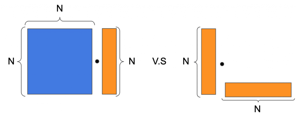
Figure 1: Two matrix/vector products consuming the same FLOPs. Left: matrix * vector product. Right: vector * vector outer product, where after the outer product we sum each of the columns.
Each of these operations consumes 2xNxN-N FLOPs, which are broken up into NxN floating-point (FP) multiplications and NxN-N FP additions.
We now consider accelerating these computations using a GPU (see Python code below). The graphs in Figure 2 depict the run-time vs. the FLOPs measured for the two operations. These graphs were generated by applying each of the products with increasing values of N, and averaging across multiple runs.
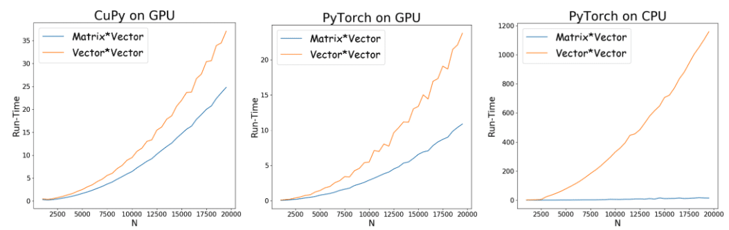
Figure 2: Run-time (in seconds) as a function of N(FLOPS =2xNx2-N) of the matrix multiplication versus vector multiplication and summation. Blue: Matrix* Vector; Orange: Vector * Vector (outer product). The X-axis (N) is the size of the vector/matrix. From left to right: CuPy on GPU, PyTorch on GPU PyTorch on CPU.
Although the number of FLOPs in each scenario is the same, their run-times differ substantially. Moreover, the difference gets larger as N(the number of entries in the matrices) increases. For example, it is evident in the CuPy curve that when the vector/matrix size is N=20,000, the outer product takes roughly 1.5 times longer than the matrix multiplication. Using PyTorch, when N=20,000, the difference becomes more than 2 times longer.
Here are some common explanations for the formidable differences in running times observed for the operations.
A lower-level view of GPU computation
To understand what can differentiate between FLOPs and run-time, we need to first understand how the GPU performs computations. Behind the scenes, there are two kinds of operations when computing the value of a layer in a deep neural network:
Multiply and accumulate (MAC) — This operation takes three inputs: kernel (or information about the kernel), input data, and partial sum computed from the previous iteration. These three inputs are transferred through the arithmetic logic unit (ALU), which performs the bit-wise operation of multiplication and addition. The output of the operation is a partial sum that is stored in a separate memory unit.
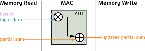
Memory access — This operation takes the partial sum computed for every MAC operation and stores it in a designated memory unit, depending on its size. Roughly speaking, there are four (sometimes more) types of memory units: the register file (RF) memory, which stores a small amount of data (up to 1Kb); the processing engine (PE), which stores a bit more data; the buffer unit; and the DRAM. As the size of the memory unit increases, the time consumption of this unit increases as well. In the worst case, reading and writing to the DRAM can be very costly and take more than 200 times to run than storing on RF.
When we count FLOPs, we don’t actually distinguish between the MAC and the memory access operations. These, however, can be very different from the running time. A sequence of MACs that require a lot of DRAM storage could take much more time than the same number of MACs that don’t use DRAM at all.
The ability to parallelize operations is another factor that can impact the final running time. In contrast to CPUs, which consist of a few cores that are optimized for sequential serial processing, GPUs consist of a massively parallel architecture containing thousands of smaller cores. This offers an advantage to network structures that can run in parallel. For example, the structure of the GPUs entails that up to a certain size, a wider and shallower network will run faster on a GPU than a deep and thin network. This occurs because the operations of the wider network can be computed in a parallel manner if they occupy more GPU cores, while the computations of the deeper network need to be done in a more sequential manner. The parallelization of the operation depends on the specific hardware and algorithmic operations used.
Going back to our numerical example, it is possible to attribute the difference in run-times to two factors: parallelism and memory accesses. That said, a custom implementation can reduce the difference in running time; hence, this difference strongly depends on the specific implementation of the framework used. We were able to identify the specific memory access and parallelism bottlenecks using an NVIDIA tool named Nsight system. We will leave that topic for a future post.
Memory-minded programming can speed up computations
Despite the significant gaps we observe in Figure 2, we would like to exemplify the impact of the framework on the results. When using high-level frameworks (e.g CuPy, PyTorch, TensorFlow, etc.), we are in fact using a predefined algorithm. In different use cases, different algorithms exhibit different performance. For instance, the CuPy implementation of a 2D array is implemented by reindexing entries of a 1D array. This implies that when trying to pop elements from the 2D array, adjacent elements in a row will be retrieved faster than adjacent elements in a column. For this reason, we can expect a generic algorithm to perform summation faster over rows than over columns. Recall that in the results in Figure 2, we performed the summation with CuPy over columns. We now show that by changing the dimension of the summation, we can (almost) make the run-time of the two operations equal. This can be seen in Figure 3:
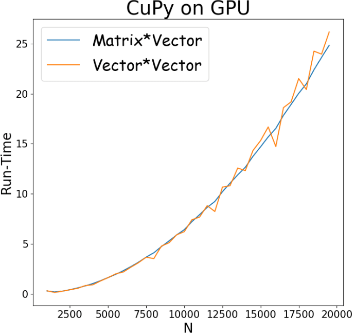
Figure 3: Run-time (in seconds) vs. FLOPs of the matrix multiplication versus vector multiplication and summation. Blue: matrix* vector; Orange: vector * vector (outer product). The X-axis corresponds to (N) the number of entries in the matrix. This implementation used CuPy, where the summation after the outer product was performed over the rows.
Although in this specific example we were able to improve the results by changing one line of code, this is not always possible when using higher-level frameworks. For example, if we try the same trick with PyTorch, the results are not improved significantly. Moreover, when it comes to real deep networks, decreasing the run-time requires very high expertise.
Conclusion
Using a concrete example of a matrix/vector product, we demonstrated that, when it comes to run-time, FLOPs cannot be used as a universal proxy for efficiency. Often this fact is overlooked, even in certain academic papers. We used CuPy and PyTorch to demonstrate how two matrix/vector multiplications, which consume precisely the same number of FLOPs, can have radically different run-times. We also briefly discussed the reasons for these differences.
CuPy Code
import cupy as cp
import time
import os
import numpy as np
import matplotlib.pyplot as plt
from cupy import cuda
import pickle

def cp_Matmul(x, y, iterations):
    for i in range(iterations):
      q = cp.matmul(x, y, out=None)
    return q

def cp_Vecmul(x,y,iterations):
    for i in range(iterations):
        q = cp.matmul(x,y,out=None)
        q = cp.sum(q,axis=1)
    return q

xmin = 1000
xmax = 20000
jump = 500
lim = range(xmin,xmax,jump)

Matrix_result = []
Vector_result = []
iterations = 1000

for k in lim:
    N = k

    vec_outer_1 = cp.random.rand(N,1)
    vec_outer_2 = cp.random.rand(1,N)

    matrix = cp.random.rand(N,N)
    vec_matrix = cp.random.rand(N,1)


    start_event = cp.cuda.stream.Event()
    stop_event = cp.cuda.stream.Event()
    start_event.record()
    q = cp_Vecmul(vec_outer_1,vec_outer_2,iterations)
    stop_event.record()
    stop_event.synchronize()
    Vector_time = cp.cuda.get_elapsed_time(start_event, stop_event)/1000
Matrix_result.append(Matrix_time)
print('Total run time matrices', Matrix_time)
PyTorch Code
import os
import numpy as np
import matplotlib.pyplot as plt
import torch
import pickle

def tr_Matmul(a, b, iterations):
    for i in range(iterations):
        q = torch.mm(a, b, out=None).to(device=cuda0)
    return q

def tr_Vecmul(a,b,iterations):
    for i in range(iterations):
        q = torch.mm(a,b,out=None).to(device=cuda0)
        q = torch.sum(q,dim=0).to(device=cuda0)
    return q

xmin = 1000
xmax = 20000
jump = 500
lim = range(xmin,xmax,jump)

Matrix_result = []
Vector_result = []
iterations = 1000

for k in lim:
    N = k
    cuda0 = torch.device(device='cuda')

    vec_outer_1 = torch.rand(N,1).to(device=cuda0)
    vec_outer_2 = torch.rand(1,N).to(device=cuda0)

    matrix = torch.rand(N,N).to(device=cuda0)
    vec_matrix = torch.rand(N,1).to(device=cuda0)


    start_event = torch.cuda.Event(enable_timing=True)
    stop_event = torch.cuda.Event(enable_timing=True)
    start_event.record()

    q = tr_Vecmul(vec_outer_1,vec_outer_2,iterations)
    stop_event.record()
    torch.cuda.synchronize()
    Vector_time = start_event.elapsed_time( stop_event)/1000
    Vector_result.append(Vector_time)
    print('Total run time vectors',Vector_time)

    start_event = torch.cuda.Event(enable_timing=True)
    stop_event = torch.cuda.Event(enable_timing=True)
    start_event.record()

    q = tr_Matmul(matrix, vec_matrix, iterations)
    stop_event.record()
    torch.cuda.synchronize()
    Matrix_time =  start_event.elapsed_time( stop_event)/1000
    Matrix_result.append(Matrix_time)
    print('Total run time matrices', Matrix_time)