Editor’s note: This post was originally published in April 2022 and has been updated for accuracy and comprehensiveness.
Introduction
Deep neural networks (DNNs), coupled with the right image data, can be used to tackle everyday real-world problems, including medical image analysis, video conferencing, or autonomous driving. However, solving these problems efficiently with AI is a challenge. In many cases, only the best, AKA state of the art (SOTA) DNNs can meet the limitations of a given application.
In this blog, we discuss the different types of DNNs currently used to tackle common computer vision tasks, including image classification, object detection, and semantic segmentation. We begin by explaining what counts as a SOTA DNN, and then survey the SOTA DNNs for each computer vision task.
What Are SOTA DNNs?
State-of-the-art (SOTA) Deep Neural Networks (DNNs) are the best models you can employ for a specific task. A DNN can earn the SOTA label based on its accuracy, speed, or any other relevant metric. However, in many computer vision domains, there exists a trade-off among these metrics. In other words, you might have a DNN that is very fast, but its accuracy falls short. Conversely, there are DNNs with impressive accuracy metrics that lack the necessary latency or throughput across various tasks, such as image classification and object detection. In these domains, a DNN will be deemed SOTA if it delivers an optimal trade-off between the relevant metrics.
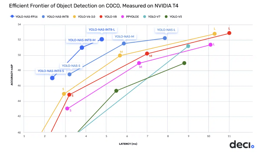
The metrics we usually use to compare and evaluate DNNs are accuracy, precision, recall, F1-score, IoU, and mAP. A DNN will be declared state-of-the-art if it delivers the best tradeoff of these metrics with additional performance metrics of interest, such as FLOPS, latency, throughput, and more. For example, in the figure above, we can see the accuracy-latency trade-off of object detection models on a specific hardware, namely NVIDIA T4. The object detection models that deliver the highest accuracy for a specific latency and vice versa are considered SOTA DNNs.
Core Architectures for Computer Vision: CNNs and ViTs
Convolutional Neural Networks (CNNs) and Vision Transformers (ViTs) are architectures commonly used in computer vision, each using a unique method of processing visual data.
- CNNs have been the cornerstone for image processing tasks. They employ convolutional layers to systematically scan images, initially detecting basic features like edges and progressively identifying more intricate patterns deeper in the network. Due to their structured approach, CNNs have excelled in tasks such as image classification and object detection.
- ViTs introduce a novel approach to image analysis. Originating from transformer architectures initially developed for natural language processing, ViTs segment images into fixed-size patches and process them as sequences, not grids. Their inherent attention mechanisms enable them to discern relationships between various patches, capturing context and offering an interpretation distinct from CNNs. This innovative perspective by ViTs has enriched the computer vision domain, igniting extensive research into synergies between them and CNNs.
Image Classification
Image classification involves training computer algorithms to automatically categorize images into predefined groups or “classes”. For instance, when presented with various animal images, the algorithm should be able to categorize them into respective classes such as “cats”, “dogs”, or “birds”. In this process, a model receives an image as input and is tasked with accurately determining its corresponding class.
How CNNs Work in Image Classification
To fathom the intricacies of Convolutional Neural Networks (CNNs) in image classification, picture an image being systematically swept by a set of tiny, overlapping windows. These windows, or filters, slide across every part of the image, looking for specific visual patterns—be it a line, curve, or texture. As the image progresses through the layers of the network, these patterns become increasingly complex: transitioning from rudimentary edges to intricate structures like eyes or feathers.
After this initial discovery of patterns, the network introduces pooling layers. Imagine these as a means to compress or ‘downsample’ the image, retaining only the most vital features and discarding redundant details, thus simplifying the information and reducing computation.
Having processed the image through these convolutional and pooling stages, the data is then flattened into a one-dimensional array and passed to what are termed fully connected layers. These layers act as the decision makers of the network, weighing the discovered patterns and features to determine the image’s category—say, distinguishing between a “cat”, a “dog”, or a “bird”.
In essence, CNNs methodically sift through an image, detect hierarchical features using convolutions, distill essential information, and employ dense layers to draw conclusions about the image’s content.
How ViTs Work in Image Classification
To grasp the workings of Vision Transformers (ViTs), envision an image being segmented into numerous small squares, akin to a mosaic or a 16×16 grid. Each of these squares is translated into a numerical representation, encapsulating all its colors (RGB values). These number sequences, known as patch embeddings, are reminiscent of how transformers represent words in a sentence.
Interestingly, the original transformer architecture doesn’t inherently preserve the sequential order of these embeddings. To address this, ViTs incorporate a positional embedding to each patch embedding, ensuring the model retains spatial awareness of each segment’s origin within the image.
With this enriched information in hand, the patch embeddings are then processed through the transformer. Leveraging its attention mechanisms and multiple layers, the transformer carefully analyzes the image’s content, eventually determining its category (e.g., discerning if the image depicts a “cat” or a “dog”).
In a nutshell, ViTs deconstruct an image into numerical representations, infuse it with spatial context, and harness the transformer’s capabilities to evaluate and classify the visual data.
Having delved into the mechanics of ViTs and CNNs for image classification, let’s now turn our attention to particular Deep Neural Networks (DNNs) designed for this task.
SOTA DNNs for Image Classification
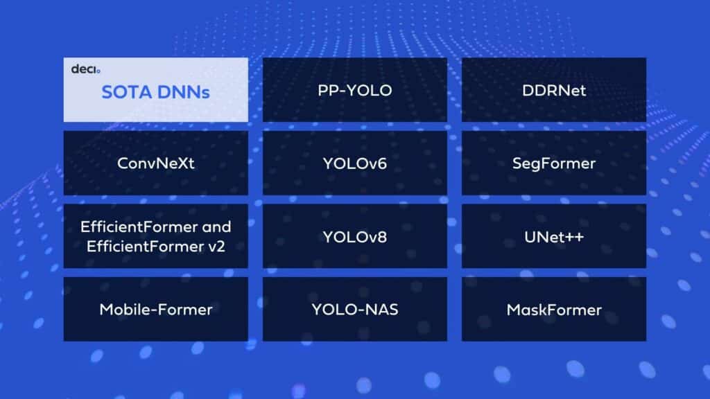
In this section, we’ll examine leading deep learning models like ConvNeXt, EfficientFormer, and MobileFormer. These models are at the forefront of image classification, each boasting unique features that optimize performance across various tasks.
ConvNeXt
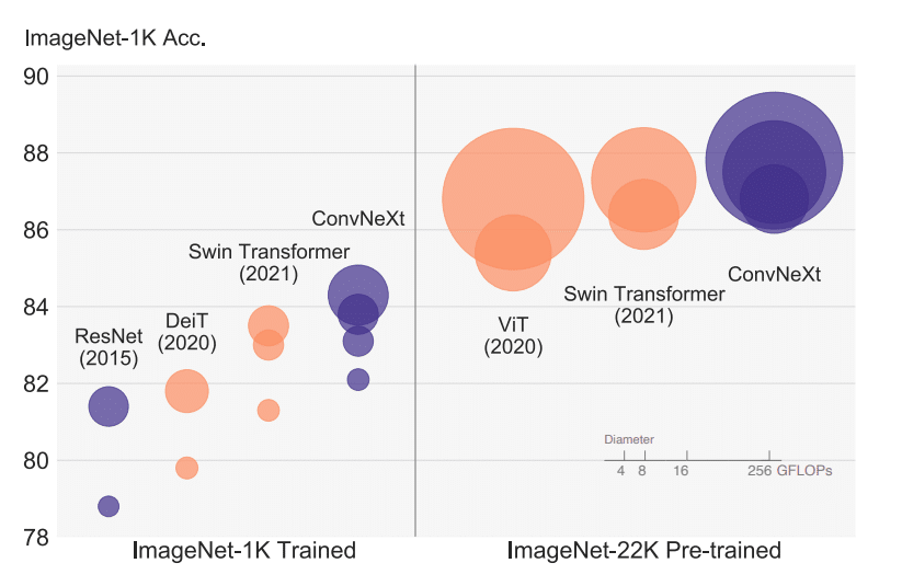
ConvNeXt rejuvenates traditional CNNs, or “ConvNets”, as highlighted in A ConvNet for the 2020s by Zhuang Liu et al. This innovative model revamps standard ConvNet architectures to compete with the prowess of Vision Transformers (ViTs) in a range of computer vision tasks. Remarkably, ConvNeXt is built solely from classical ConvNet modules, merging simplicity and efficiency without compromising on performance. It achieves an impressive 87.8% top-1 accuracy on ImageNet and surpasses Swin Transformers in tasks like COCO object detection and ADE20K semantic segmentation.
Its architectural evolution starts from a base ResNet and integrates elements reminiscent of a Vision Transformer, incorporating design principles from ResNeXt, inverted bottleneck structures, and employing enlarged kernel sizes. These modifications bridge the performance chasm between traditional ConvNets and cutting-edge Transformers. As a result, ConvNeXt showcases performance metrics comparable to or even surpassing Transformers, all while staying true to its ConvNet heritage
What sets ConvNeXt apart is its capability to achieve stellar performance without the attention mechanisms characteristic of Transformers. Instead, it smartly navigates the design avenues that underpin Transformer success, leveraging purely convolutional means. Beyond its noteworthy ImageNet accuracy, ConvNeXt excels in diverse vision tasks, even outpacing established models like Swin Transformers. All this, while preserving the hallmark simplicity and computational efficiency of ConvNets.
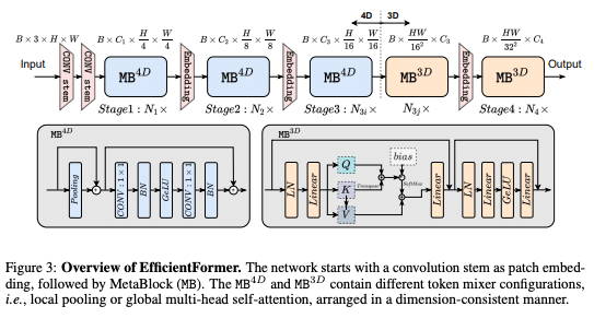
EfficientFormer and EfficientFormer v2
EfficientFormer and its successor, EfficientFormer v2, represent breakthroughs in DNNs, showcasing the potential of mobile-optimized Vision Transformers (ViTs). These models deftly combine the robustness of ViTs with the essential efficiency required for mobile device deployment.
The original EfficientFormer adopts a unique dimension-consistent design, eliminating frequent reshaping operations, which reduces computational costs. EfficientFormer v2 further hones this approach, leveraging a supernet and a fine-grained joint search strategy to strike an optimal balance between latency and parameter efficiency. The models span multiple sizes: EfficientFormer ranges from L1 to L7, while EfficientFormer v2 offers variants like S0 and S1, each meticulously designed for a specific blend of accuracy and efficiency.
What sets EfficientFormer apart is its innovative design that prioritizes on-device speed, while EfficientFormerV2 optimizes architecture for increased accuracy without added latency. It does so by unifying the Feed Forward Network (FFN) and innovating the Multi Head Self Attention (MHSA) mechanism.
In performance terms, both versions strike an admirable balance between speed and accuracy, crucial for mobile deployment. EfficientFormer’s L1 model boasts a 79.2% top-1 accuracy on ImageNet-1K with a swift 1.6 ms inference time on an iPhone 12. EfficientFormerV2’s S0 model outperforms MobileNetV2, achieving a 3.5% higher top-1 accuracy on ImageNet-1K with comparable latency and parameters. These advancements underscore the feasibility of integrating efficient, high-performing vision transformers into mobile platforms without compromising on performance.
Mobile-Former
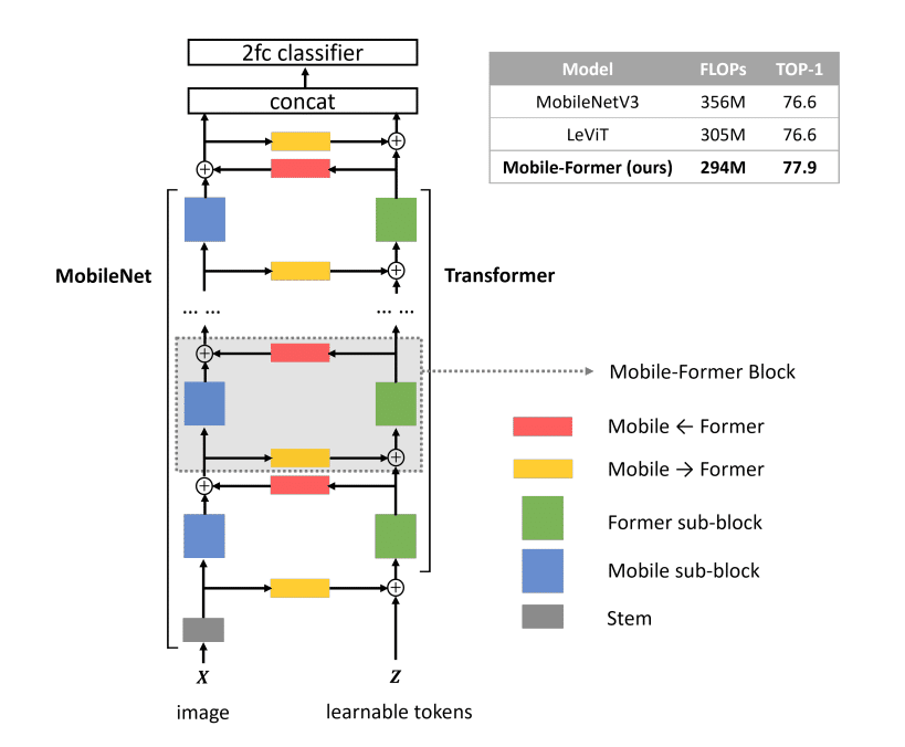
Mobile-Former, introduced in Mobile-Former: Bridging MobileNet and Transformer, innovatively combines the strengths of MobileNet and Transformer models to produce an architecture that stands out in efficiency and performance. By utilizing MobileNet for adept local processing and leveraging a Transformer for nuanced global interaction, this architecture benefits from a unique bidirectional bridge that ensures a seamless fusion of both local and global features. What sets the Transformer aspect of this design apart is its minimalistic approach, using a very limited number of tokens, which drastically cuts computational overheads.
Central to Mobile-Former’s innovation is its ability to effectively harness both local and global features. While MobileNet focuses on efficient local feature extraction, the Transformer captures broader interactions. Their connection through a bidirectional bridge facilitates the exchange and enrichment of these features, further enhanced by a lightweight cross attention mechanism.
Performance metrics of Mobile-Former are impressive. In the realm of image classification, it achieves a 77.9% top-1 accuracy on the ImageNet dataset at 294M FLOPs, surpassing the benchmarks set by MobileNetV3. When evaluated in object detection tasks, Mobile-Former demonstrates superior capability, outclassing MobileNetV3 within the RetinaNet framework by an 8.6 Average Precision (AP) margin. Notably, when incorporated into the DETR framework as the backbone, encoder, and decoder, it not only outperforms DETR with a 1.1 AP lead but also achieves a 52% reduction in computational cost and a 36% decrease in the number of parameters.
In conclusion, Mobile-Former presents itself as a groundbreaking architecture that deftly marries the best of MobileNets and Transformers, promising exceptional efficiency without compromising on performance.
Object Detection
Object detection stands as a cornerstone of computer vision, tasked with identifying and pinpointing objects within images. It goes beyond mere object recognition, offering a dual perspective by identifying both the type of object (“what”) and its specific location within the image (“where”), often represented by bounding boxes. Two predominant methodologies are central to object detection tasks: Single Shot Detection (SSD) and Two-Stage Networks.
(i) Single Shot Detection (SSD): Designed with efficiency in mind, SSD executes object detection in just one forward pass through the network. Instead of treating object localization and classification as separate tasks, SSD integrates them, yielding a streamlined and rapid detection process. Here, images are divided into grids, with bounding boxes and class probabilities predicted simultaneously. The result? Faster object detection that’s gentler on computational resources.
(ii) Two-Stage Networks: A bit more intricate, this approach is divided into two main steps. Initially, a Region Proposal Network (RPN) examines the image to suggest potential bounding boxes, spotlighting areas likely containing objects. Following this, a second, separate CNN refines these proposals and takes on the task of object classification. Although this method tends to be more accurate, its bifurcated nature makes it more computationally intensive compared to SSD.
The choice between SSD and Two-Stage Networks often boils down to the specific needs of an application. While SSDs are favored in scenarios where real-time processing and low latency are paramount, Two-Stage Networks are sought after when precision takes precedence. Nonetheless, advancements in SSD have enabled it to deliver competitive performance metrics while consuming fewer computational resources, positioning it as a preferred choice for many real-time and resource-limited applications.
SOTA DNNs for Object Detection
Among the myriad of object detection models, PP-YOLO, YOLOv6, YOLOv8, and YOLO-NAS stand out as leading SOTA DNNs. Each model brings its own set of architectural advancements and performance improvements to the table. In this section, we offer a concise examination of these standout models, highlighting their architecture, key features, and performance benchmarks.
PP-YOLO
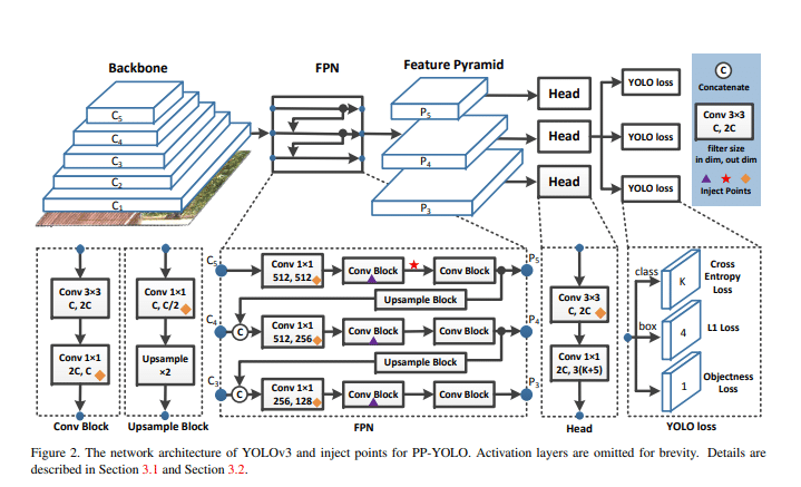
Based on the YOLO (You Only Look Once) SSD architecture, PP-YOLO stands as a notable advancement in object detection, adeptly striking a balance between effectiveness and efficiency. Introduced in the research paper PP-YOLO: An Effective and Efficient Implementation of Object Detector, the model builds upon the YOLOv3 architecture but optimizes it further by amalgamating several existing methodologies. This enhancement strategy bolsters detection accuracy without notably compromising the model’s speed. With an impressive mean average precision (mAP) of 45.2% and a swift processing rate of 72.9 FPS, PP-YOLO not only holds its own but even outperforms distinguished models like EfficientDet and YOLOv4.
At its core, PP-YOLO embodies a blend of simplicity and effectiveness. It employs a tailored version of the ResNet architecture, specifically the ResNet50-vd-dcn, complemented by a Feature Pyramid Network (FPN) for adept image data processing. Its detection head is streamlined, consisting of just two convolutional layers. By judiciously adopting various existing techniques, PP-YOLO fine-tunes its parameters and FLOPs to achieve heightened accuracy while preserving a similar speed to its foundational model.
What sets PP-YOLO apart is its innovative incorporation of several performance-enhancing methodologies without unduly taxing efficiency. These include the Grid Sensitive approach for more accurate bounding box predictions, Matrix NMS for accelerated processing, and both CoordConv and Spatial Pyramid Pooling (SPP) to elevate detection capabilities. Additionally, by leveraging larger batch sizes and integrating an Exponential Moving Average (EMA), PP-YOLO refines its detection capabilities without placing undue strain on computational resources, marking it as a sophisticated evolution in object detection technology.
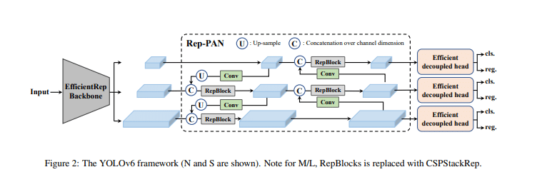
YOLOv6
YOLOv6, stemming from the lineage of the renowned YOLO series, introduces an innovative architecture characterized by an efficient backbone, a PAN (Pyramid Attention Network) topology neck, and a uniquely efficient decoupled head. The backbone, fortified with RepVGG or CSPStackRep blocks, boosts feature extraction, while the PAN neck capitalizes on multi-scale features—essential for detecting objects of various sizes. The decoupled head, utilizing a hybrid-channel approach, optimizes detection through varied channel-wise operations.
YOLOv6 stands out for its adoption of advanced quantization methods, including post-training quantization and channel-wise distillation. These techniques enhance the model’s performance in resource-constrained environments, ensuring high accuracy without significant compromises.
YOLOv6 sets new benchmarks, outstripping models like YOLOv5, YOLOX, and PP-YOLOE in both accuracy and processing speed. Its meticulously designed architecture, coupled with cutting-edge quantization strategies, positions YOLOv6 as a leading choice for real-time object detection endeavors.
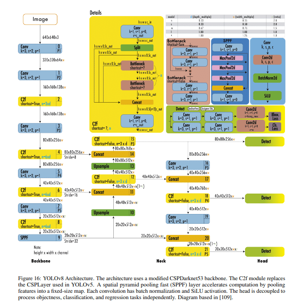
YOLOv8
Introduced by Ultralytics in January 2023, YOLOv8 stands out as a versatile and scalable object detection model. It’s available in five variants: YOLOv8n, YOLOv8s, YOLOv8m, YOLOv8l, and YOLOv8x, designed to address a range of computational demands and application scenarios.
In terms of architecture, YOLOv8 utilizes a backbone reminiscent of YOLOv5, but it’s enriched by the C2f module. This module boosts detection accuracy by fusing high-level features with contextual insights. The model’s anchor-free approach, combined with a decoupled head, optimizes the handling of objectness, classification, and regression tasks. With the integration of CIoU and DFL loss functions tailored for detecting smaller objects, as well as binary cross-entropy for classification loss, YOLOv8 reflects a notable advancement in object detection capabilities.
Demonstrating its prowess, YOLOv8x achieved a notable 53.9% AP on the MS COCO dataset with a 640-pixel image size, operating at a swift 280 FPS on an NVIDIA A100 with TensorRT. This emphasizes YOLOv8’s proficiency in delivering both accuracy and speed.
YOLO-NAS
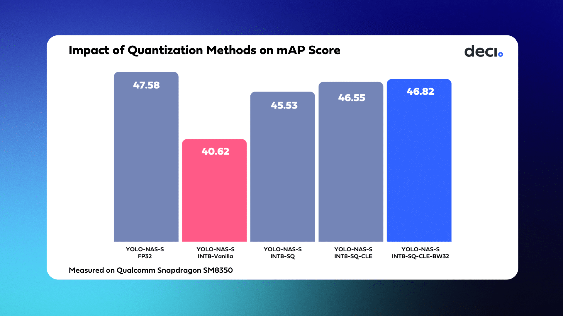
Released in May 2023 by Deci, YOLO-NAS is a pioneering architecture in the domain of object detection setting unparalleled standards in balancing accuracy and latency. It incorporates QSP and QCI blocks, which meld the benefits of re-parameterization and 8-bit quantization, ensuring minimal accuracy degradation during post-training quantization. Deci’s proprietary neural architecture search (NAS) technology, AutoNAC, was instrumental in generating the YOLO-NAS architecture. It determined the optimal sizes, block types, number of blocks, and channel counts in every stage.
Rather than adopting a standard quantization approach, which can result in notable accuracy loss, YOLO-NAS introduces a hybrid quantization technique. This method selectively quantizes specific portions of the model based on an advanced layer selection algorithm, optimizing the balance between latency and accuracy. The algorithm meticulously evaluates the impact of each layer on overall performance, as well as the effects of alternating between 8-bit and 16-bit quantization.
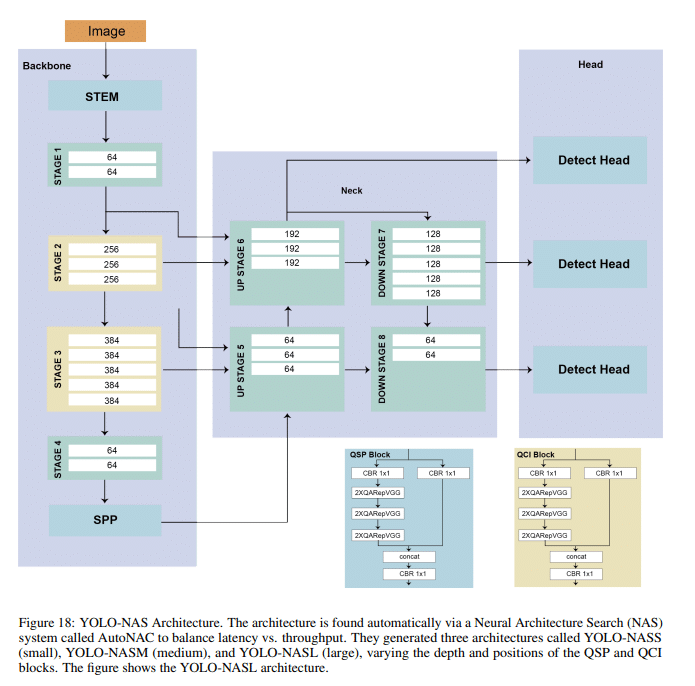
Designed with production in mind, YOLO-NAS is tailored to seamlessly integrate with high-end inference engines like NVIDIA® TensorRT™, and it supports INT8 quantization for unmatched runtime performance. Its adaptability positions it as an optimal choice for real-world applications that demand low latency and robust processing, such as autonomous vehicles, robotics, and video analytics.
The architecture further innovates by employing state-of-the-art techniques like attention mechanisms, quantization-aware blocks, and reparametrization during inference. These elements empower YOLO-NAS to adeptly detect objects, regardless of their size or intricacy, redefining excellence in the object detection landscape and its applicability across various industries.
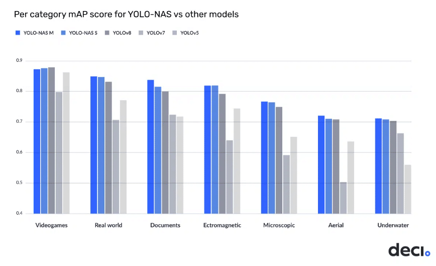
The YOLO-NAS architecture represents the pinnacle of efficiency in object detection tasks, delivering an unparalleled balance between accuracy and latency, as illustrated in the following graph:
YOLO-NAS was trained using the RoboFlow100 dataset (RF100), a compilation of 100 datasets spanning varied domains, to exhibit its proficiency in intricate object detection challenges. The RF100 dataset serves as a standard for existing YOLO models. This training allowed for a direct comparison of YOLO-NAS’s performance with YOLO versions v5, v7, and v8, highlighting its superiorities. A detailed, category-wise performance analysis of YOLO-NAS on the RF100 dataset vis-à-vis the v5/v7/v8 models follows.
Semantic Segmentation
Semantic segmentation is a pivotal technique within computer vision, where each pixel of an image is assigned a class label. More than just recognizing and locating objects, it meticulously delineates an object’s boundaries down to the pixel level. This high granularity of classification has made semantic segmentation invaluable in myriad applications across diverse domains. In the context of autonomous vehicles, it provides an acute understanding of the driving environment by precisely segmenting each element, such as roads, vehicles, and pedestrians, ensuring safer navigation. In the medical realm, semantic segmentation aids in pinpointing and demarcating specific regions of interest, like tumors or other pathological structures, furnishing essential insights for diagnosis and treatment. Video conferencing applications harness semantic segmentation to enable features like background blur or virtual background, accurately distinguishing participants from their backdrop.
SOTA DNNs for Semantic Segmentation
The application of Deep Neural Networks (DNNs) in semantic segmentation has ushered in remarkable advancements, offering robust models capable of astute pixel-level classification across varied applications. Let’s delve into a few state-of-the-art DNNs that have significantly impacted semantic segmentation in different fields:
Autonomous Vehicle Applications
DDRNet
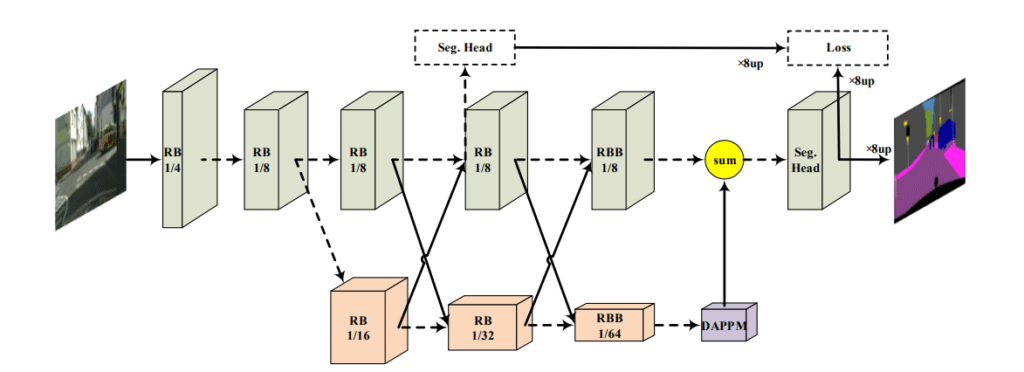
DDRNet, or Dual-Resolution Networks, introduces a compelling approach to semantic segmentation, particularly for high-resolution images common in road-driving contexts. This intricate deep learning network ingeniously bifurcates into two distinct branches. The first branch is dedicated to generating high-resolution feature maps, while the second delves deeper, employing multiple downsampling operations to extract essential semantic information.
A distinguishing facet of DDRNet is its Deep Aggregation Pyramid Pooling Module (DAPPM). This component processes low-resolution feature maps to extract multi-scale contextual data and seamlessly amalgamates them using a cascading structure. DDRNet also incorporates multiple bilateral fusion operations between its two core branches, ensuring optimal information integration. This design choice strikes a commendable equilibrium between precise segmentation and inference speed.
In terms of performance, DDRNet offers a spectrum of models, each balancing speed and accuracy. For instance, DDRNet-23-slim achieves a mIoU of 77.4% on the Cityscapes test set, with an impressive 102 FPS. In contrast, the more robust DDRNet-39 1.5x registers a stellar 82.4% mIoU, underscoring its heightened accuracy. This versatile performance across different model sizes harmonizes computational efficiency with segmentation precision, making it suitable for a wide range of real-time applications.
SegFormer
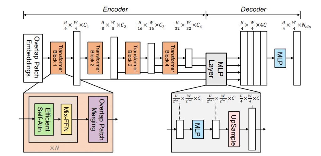
SegFormer stands out as a novel Transformer framework meticulously designed for semantic segmentation. By seamlessly integrating Transformers with lightweight multilayer perceptron (MLP) decoders, it delivers a unified solution tailored for this task. At the core of its architecture is a hierarchically structured Transformer encoder, capable of producing multi-scale features. Intriguingly, this encoder sidesteps the usual need for positional encoding, thus eliminating the challenges associated with interpolating positional codes. This design ensures the model’s effectiveness remains uncompromised, even when the test resolution differs from the training setup.
SegFormer is defined by two standout innovations:
- The hierarchical Transformer encoder, which is devoid of positional encoding, masterfully outputs a range of features, spanning from detailed high-resolution to broader low-resolution. Its absence of positional encoding becomes especially advantageous when the image resolution during inference is distinct from the training phase.
- The all-MLP decoder, on the other hand, skillfully integrates information from multiple layers. Harnessing both local and global attention mechanisms, it crafts powerful representations without resorting to complex designs, thus emphasizing efficiency.
When it comes to the balance of speed and accuracy, SegFormer truly excels. It introduces a diverse array of models from SegFormer-B0 to SegFormer-B5, each calibrated for a unique balance between performance and efficiency. A testament to its capabilities, the SegFormer-B4 model achieves a commendable 50.3% mIoU on the ADE20K dataset with only 64M parameters. This makes it five times more compact yet 2.2% more effective than the prior best-performing method. Overall, with its remarkable blend of accuracy, speed, and efficiency, SegFormer sets a new gold standard on several widely-acknowledged semantic segmentation datasets.z`za
Medical and conference applications
UNet++
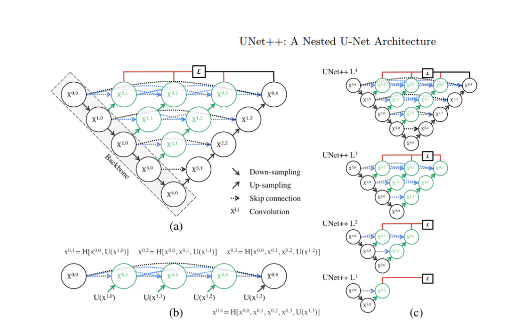
UNet++ stands out in medical image segmentation, utilizing a deeply-supervised encoder-decoder network with innovative nested and dense skip pathways. These pathways intricately connect encoder and decoder sub-networks, aiming to alleviate the semantic gap between their respective feature maps. The architecture uniquely allows operation in two distinct modes – a precision-oriented mode using all segmentation branches and a rapid mode utilizing a singular segmentation branch.
Pivoting on innovative features, UNet++ employs redesigned skip pathways which utilize a dense convolution block to semantically enhance encoder feature maps before merging with decoder maps. Nested and dense skip connections act to diminish the semantic gap between the encoder and decoder feature maps, simplifying the optimizer’s learning task. Deep supervision facilitates a choice between accuracy and speed, also allowing for strategic model pruning.
Demonstrating adept performance, UNet++ achieves notable average IoU gains over its predecessors, U-Net and wide U-Net, across various medical segmentation tasks. It not only offers a pragmatic approach to balance between accuracy and inference speed through model pruning but also showcases an impressive ability to reduce inference time with minimal impact on accuracy, embodying a practical choice in medical image segmentation applications.
Instance Segmentation
Building upon the foundation of semantic segmentation, where each pixel in an image is classified to a specific category, instance segmentation introduces a deeper granularity to this process. While semantic segmentation efficiently classifies pixels into categories, it treats all objects of the same category as a collective whole, without differentiating between individual objects.
Instance segmentation rises to this challenge. It not only classifies pixels according to their corresponding categories but also differentiates between individual objects within those categories. For example, in a scene with multiple pedestrians, while semantic segmentation would label all pedestrians under a unified ‘pedestrian’ category, instance segmentation would delineate each pedestrian separately. This allows for the identification of each unique ‘instance’ of the pedestrian category.
In this way, instance segmentation marries the strengths of object detection, which identifies distinct objects, with those of semantic segmentation, which categorizes pixels. The result is a nuanced understanding of images where each distinct object, even if it belongs to the same category as others, is recognized and segmented individually.
MaskFormer
Segmentation models have typically operated within the confines of specific tasks—semantic or instance-level segmentation. MaskFormer proposes a deviation from this norm by introducing an integrated approach.
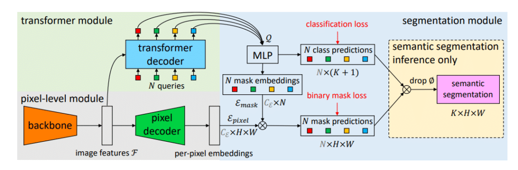
MaskFormer is a mask classification model that employs a pixel-level module combined with a Transformer decoder. This combination enables it to generate both per-pixel and per-segment embeddings. It’s designed to handle both semantic and instance-level segmentation without being tied to a specific model size or variant. To further refine the embeddings, a segmentation module has been incorporated, which aims to produce accurate binary mask predictions.
Rather than focusing on per-pixel classification or instance-level segmentation separately, MaskFormer aims to streamline these processes. It predicts a set of binary masks, with each mask being associated with a single global class label. This approach seeks to simplify the segmentation processes. Additionally, the framework is designed in a way that it can convert existing per-pixel classification models into mask classification models, suggesting adaptability.
On the ADE20K dataset, MaskFormer achieves a mean Intersection over Union (mIoU) of 55.6. On the COCO dataset, it registers a Panoptic Quality (PQ) score of 52.7. When compared to traditional per-pixel classification models, MaskFormer has shown a difference of 2.1 mIoU on ADE20K. In terms of computational efficiency, there’s a noted reduction in parameters and FLOPs by 10% and 40% respectively.
The Future of SOTA DNNs: Efficiency at the Heart of Innovation
Deep Neural Networks (DNNs) have advanced significantly, with models like ConvNeXt, EfficientFormer, and MobileFormer highlighting progress in image classification, and YOLO variants, DDRNet, and SegFormer marking achievements in object detection and semantic segmentation. A dominant theme is the imperative of efficiency, both in model design and in real-world deployment scenarios.
Deci’s AutoNAC represents a pivotal shift in this direction. It not only expedites the DNN development process by tailoring architectures to specific benchmarks and data characteristics without exhaustive training but also results in models that are inherently more efficient in performance and computational demands. Given the challenges in transitioning many manually designed models to production, tools like AutoNAC suggest a future characterized by swift, targeted model design that yields DNNs optimized for deployment.
In summary, the trajectory of DNNs is increasingly geared towards blending advanced capabilities with practical deployment efficiency. As AI evolves, the spotlight will be on tools and strategies that further hone this synergy.