How to Instruction Tune DeciLM 6B using QLoRA

Introduction

While large language models (LLMs) have “learned” a lot during their pretraining, their vast knowledge often lacks the fine edge of specialization for niche tasks. This is where fine-tuning comes into play, tailoring these models to specific needs. However, fine-tuning has its costs, especially with the hefty size of modern LLMs. The QLoRA paper (which stands for Quantized Low Rank Adaptation) proposes a method that significantly reduces memory usage, which allows the fine-tuning of LLMs to become more accessible and efficient.

By slashing resource requirements, QLoRA paves the way for broader experimentation and development, enabling researchers and practitioners with limited resources to participate in advancing the field. In fact, the findings in this paper make it possible to fine-tune a 65B parameter model on a single 48GB GPU while preserving performance.

But, how does the QLoRA magic work?

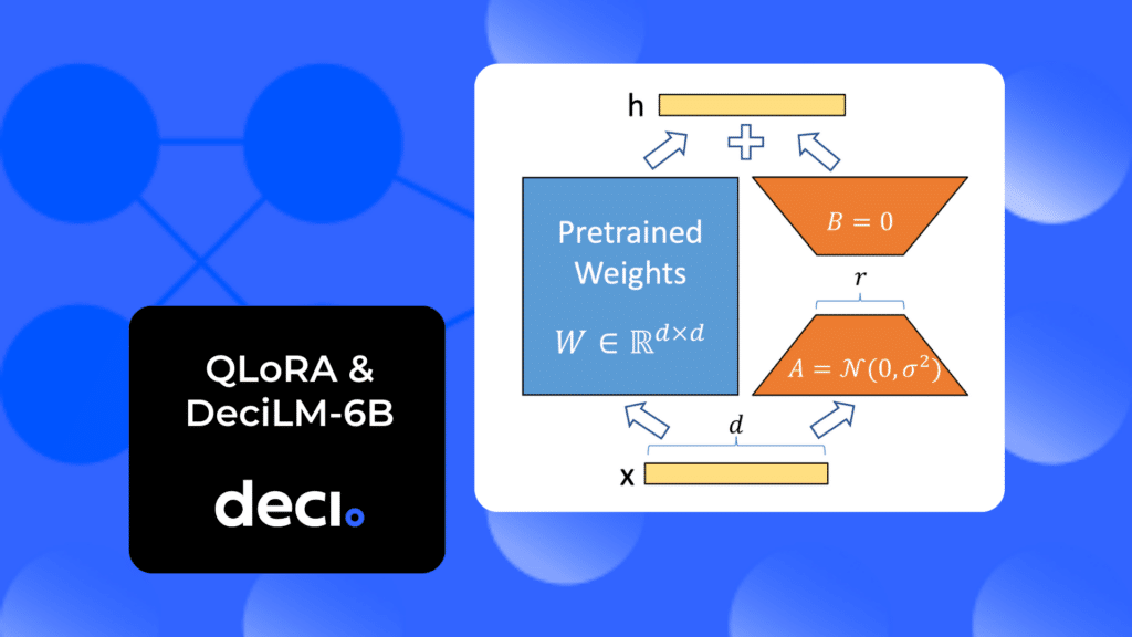
QLoRA uses Low Rank Adaptation (LoRA), a technique that modifies a compact set of model parameters, maintaining the majority untouched.

LoRA operates under the hypothesis that weight changes during model adaptation are inherently of low rank, meaning that only a subset of features needs emphasizing during fine-tuning.

The rank of a matrix informs the dimensions of the space its columns generate. It’s dictated by the number of linearly independent rows or columns.

Here’s a quick breakdown of LoRA:

• The rank of a matrix tells us the dimensions of the space spanned by its columns (or rows), which is determined by the number of linearly independent columns (or rows) in the matrix.
• A full-rank matrix has a rank that is equal to the smaller of the number of its rows or columns, which means all the rows (or columns) are linearly independent of each other.
• A low-rank matrix has a rank that is less than the smaller of its row or column counts, indicating that some of the rows (or columns) can be expressed as a linear combination of others, and therefore, the matrix is rank-deficient.

In the context of QLoRA, the concept of low-rank adaptation involves representing the weight updates during fine-tuning as low-rank matrices.

This effectively reduces the computational resources needed because it focuses on adjusting a smaller, more significant subset of the model’s parameters rather than the entire set.

By constraining the rank of the update matrix (ΔW) to a product of two smaller matrices, QLoRA cleverly updates only a fraction of the weights, optimizing the fine-tuning process. Effectively, the QLoRA system backpropagates gradients through a frozen, quantized model into Low Rank Adapters (LoRA).

QLoRA introduces several innovations:

• 4-bit NormalFloat (NF4): The 4-bit NormalFloat is a new data type that helps maintain 16-bit performance levels. It is particularly effective in contexts where weights are normally distributed—a common characteristic in neural networks—due to its capability to maintain the performance of 16-bit floating-point representations while using only a quarter of the bits. This efficiency is achieved by using a floating-point-like format that includes a shared exponent across a block of parameters and a 4-bit mantissa for each parameter. The shared exponent allows for a dynamic range similar to that of higher bit-width formats, and the balanced assignment of bit patterns to mantissa values ensures that the quantization error is minimized across the typical distribution of weight values.
  
  

• Double Quantization: Performing double quantization is a simple yet somewhat “silly” (Tim’s words, not mine) technique. This is a trick that makes 16-bit -> 4-bit quantization more efficient. It involves adding a second quantization that quantizes the quantization constants. By applying quantization twice—first to the network parameters and then to the quantization levels themselves—the method significantly reduces the bit requirements for the quantization constants. While it may seem counterintuitive to quantize already quantized values, this process leverages the redundancy in quantization levels to further compress the model without a substantial loss in performance. In practical terms, this technique can reduce the storage and bandwidth needs of the quantization indices from an overhead of 0.5 bits per parameter to just 0.125 bits per parameter. When applied to 16-bit to 4-bit quantization scenarios, double quantization provides massive improvements in storage efficiency while maintaining the computational performance of the quantized model.
  
  

• Paged Optimizers: These optimizers are a memory-saving technique that offloads small pages automatically in the background. They are adaptive and perfect for surviving memory spikes. If you have enough memory, everything stays on the GPU and is fast. But if you hit a large mini-batch, the optimizer is evicted to the CPU and returned to the GPU later. This manages memory spikes during training.
  
  

These innovative techniques are what make it possible to fit large models onto small GPUs easily.

When stacked against traditional full-model fine-tuning, QLoRA stands out for its efficiency. It maintains performance while being significantly more resource-friendly. This means that even individuals and organizations without access to high-end computing power can now fine-tune LLMs effectively, breaking down barriers in the field.

QLoRA is a game-changer for limited budgets due to its ability to fine-tune large language models (LLMs) on a single GPU:

• Cost-Effective: Enables fine-tuning of LLMs on consumer-grade GPUs, avoiding the need for expensive, high-end hardware.
• Single-GPU Efficiency: Makes it possible to train sophisticated models on just one GPU, reducing hardware investments.
• Operational Savings: Lowers ongoing costs like electricity due to less demanding hardware requirements.
• Faster Development: Accelerates the fine-tuning process, reducing time-to-market and associated costs.
• Strategic Advantage: Provides a competitive edge by offering advanced AI capabilities without significant financial outlay.

Here’s what you need to get started fine-tuning with QLoRA using HuggingFace’s SFTTrainer:

• A language model
• A tokenizer
• A dataset
• Two configuration files: BitsAndBytesConfig and LoraConfig
• You’ll also need to use the prepare_model_for_kbit_training and get_peft_model functions from the peft library to, well prepare your model and get it into a peft format.
• And, training parameters for the SFTTrainer

Time to get into it!

First, just a couple of preliminaries.

• Set the UTF encoding for the environment so that peft doesn’t yell at you during installation.
• Create a directory for checkpoints
• Install libraries that you will need
• Log into HuggingFace so you can immediately push the trained model to the hub without baby sitting the notebook
  
  

import os
os.environ['LC_ALL'] = 'en_US.UTF-8'
os.environ['LANG'] = 'en_US.UTF-8'
os.environ['LC_CTYPE'] = 'en_US.UTF-8'

from huggingface_hub import notebook_login
notebook_login()

from pathlib import Path
from typing import Optional

def create_directory(path: Optional[Path] = None, dir_name: str = "output"):
    """
    Creates a directory at the specified path with the given directory name.
    If no path is provided, the current working directory is used.

    Parameters:
    - path (Optional[Path]): The path where the directory is to be created.
    - dir_name (str): The name of the directory to create.

    Returns:
    - Path object representing the path to the created directory.
    """
    # Use the current working directory if no path is provided
    working_dir = path if path is not None else Path('./')

    # Define the output directory path by joining paths
    output_directory = working_dir / dir_name

    # Create the directory if it doesn't exist
    output_directory.mkdir(parents=True, exist_ok=True)

    return output_directory

output_dir = create_directory(dir_name="peft_lab_outputs")
print(f"Directory created at: {output_dir}")

Directory created at: peft_lab_outputs

!pip install -qq git+https://github.com/huggingface/peft.git
!pip install -qq accelerate
!pip install -qq datasets
!pip install -qq trl
!pip install -qq transformers
!pip install -qq bitsandbytes
!pip install -qq safetensors
# note: flash attention installation can take a long time
!pip install flash-attn --no-build-isolation

  Installing build dependencies ... done
  Getting requirements to build wheel ... done
  Preparing metadata (pyproject.toml) ... done
Requirement already satisfied: flash-attn in /usr/local/lib/python3.10/dist-packages (2.3.3)
Requirement already satisfied: torch in /usr/local/lib/python3.10/dist-packages (from flash-attn) (2.1.0+cu118)
Requirement already satisfied: einops in /usr/local/lib/python3.10/dist-packages (from flash-attn) (0.7.0)
Requirement already satisfied: packaging in /usr/local/lib/python3.10/dist-packages (from flash-attn) (23.2)
Requirement already satisfied: ninja in /usr/local/lib/python3.10/dist-packages (from flash-attn) (1.11.1.1)
Requirement already satisfied: filelock in /usr/local/lib/python3.10/dist-packages (from torch->flash-attn) (3.13.1)
Requirement already satisfied: typing-extensions in /usr/local/lib/python3.10/dist-packages (from torch->flash-attn) (4.5.0)
Requirement already satisfied: sympy in /usr/local/lib/python3.10/dist-packages (from torch->flash-attn) (1.12)
Requirement already satisfied: networkx in /usr/local/lib/python3.10/dist-packages (from torch->flash-attn) (3.2.1)
Requirement already satisfied: jinja2 in /usr/local/lib/python3.10/dist-packages (from torch->flash-attn) (3.1.2)
Requirement already satisfied: fsspec in /usr/local/lib/python3.10/dist-packages (from torch->flash-attn) (2023.6.0)
Requirement already satisfied: triton==2.1.0 in /usr/local/lib/python3.10/dist-packages (from torch->flash-attn) (2.1.0)
Requirement already satisfied: MarkupSafe>=2.0 in /usr/local/lib/python3.10/dist-packages (from jinja2->torch->flash-attn) (2.1.3)
Requirement already satisfied: mpmath>=0.19 in /usr/local/lib/python3.10/dist-packages (from sympy->torch->flash-attn) (1.3.0)

from transformers import AutoModelForCausalLM, AutoTokenizer, BitsAndBytesConfig
from trl import SFTTrainer
import torch

BitsAndBytesConfig

This configuration below is literally the only thing that differentiates LoRA from QLoRA.

But what does it all mean?

Remember above when we talked about the innvoations that QLoRA introduced? Well, you don’t have to code them by hand. It’s literally just flags in a config file!

• load_in_4bit: this enables 4-bit quantization. It replaces the Linear layers with, in this case, NF4 layers from bitsandbytes.
• 4-bit NormalFloat is set with the following flag bnb_4bit_quant_type = "nf4" This sets the quantization data type in the bnb.nn.Linear4Bit layers.
• Double Quantization is set with bnb_4bit_use_double_quant=True.This allows for nested quantization where the quantization constants from the first quantization are quantized again.
• bnb_4bit_compute_dtype=torch.bfloat16let’s us use Bfloat16, a 16-bit binary floating-point number format. It’s similar to the standard 32-bit floating-point format but uses fewer bits, so it takes up less space in computer memory. The “b” in bfloat16 stands for “brain,” which refers to its use in artificial intelligence applications. This format is particularly useful for deep learning because it provides a good balance between precision and performance, allowing neural networks to run faster while still producing accurate results.
  
  

bnb_config = BitsAndBytesConfig(
    load_in_4bit = True,
    bnb_4bit_use_double_quant=True,
    bnb_4bit_quant_type="nf4",
    bnb_4bit_compute_dtype=torch.bfloat16
)

Load model

We’re using DeciLM-6B for this tutorial, because you’re on the Deci website reading a blog made by a Deci employee..so, makes sense!

Load the model with the configuration you defined above by passing it to the quantization_config argument.

You can use Flash Attention 2 by setting use_flash_attention_2=True.

Flash Attention 2 is an improved version of Flash Attention. It focuses on the part of the model called “attention,” which helps the model to focus on the most important parts of the data, just like when you pay attention to the most important parts of a lecture. Flash Attention 2 makes this process faster and uses less memory, so models can learn from larger amounts of data or run on devices with less computing power.

This is especially useful in models that need to understand or generate human language by focusing on the right words or phrases at the right time.

model_name = "Deci/DeciLM-6b"

decilm_6b = AutoModelForCausalLM.from_pretrained(
    model_name,
    quantization_config = bnb_config,
    device_map = "auto",
    use_cache=False,
    trust_remote_code=True,
    use_flash_attention_2=True
)

tokenizer = AutoTokenizer.from_pretrained(model_name)

tokenizer.pad_token = tokenizer.eos_token

tokenizer.padding_side = "right"

Data

One of the findings that Tim Dettmers, lead author of the QLoRA paper, found was that more data doesn’t beat better data.

Data Quality > Data Quantity™️

Tim Dettmers

In the paper they found using a 9k sample dataset of high quality instructions beat using a 1M dataset of mediocre quality data. For this tutorial we’ll use a highly curated datastet that I put together. This dataset was something I initially curated for entry into the NeurIPS Challenge, but ultimately didn’t enter.

It’s a mash up of 12 very high quality instruction datasets that I found on HuggingFace. Each of the sub-datasets are all permissively licensed and adhere to the challenges rules, which were as follows:

• Any generated llm dataset must be generated from one of the approved base models
• You can under no circumstance use datasets generated by ChatGPT
• You can generate a dataset with Llama2 if you make sure that your >dataset is released with the Llama2 license and if in your submission the generated dataset is only consumed by Llama2. Other models have similar licenses like qwen
• You can generate a dataset using internlm (apache 2 license) to finetune any other LLM on the approved model list

The entire dataset is >3.4M examples, and has approximately 3:2 ratio of code/non-code instructions.

It will take a bit of time to download, so feel free to swap out the dataset for whatever you’d like.

from datasets import load_dataset

dataset = "TeamDLD/neurips_challenge_dataset"

data = load_dataset(dataset)

Here’s I’m just creating a flag to indicate which dataset is code vs non-code, as well as preparing the instruction string.

def add_type(example):
    """
    Adds a 'type' field to the dataset example based on the 'source' field and the provided mapping.

    Parameters:
    - example (dict): A dictionary representing a row in the dataset.

    Returns:
    - dict: The updated dictionary with a new 'type' field.
    """
    # Retrieve the type based on the 'source' field using the mapping dictionary
    example['type'] = source_to_type.get(example['source'], 'unknown')
    return example

def example_formatter(example):
    """
    Joins the three columns 'instruction', 'input', and 'response' into a list of strings,
    with each part separated by a newline character. If 'input' is None, it is replaced
    with "### Input:\n".

    Parameters:
    - example (dict): A dictionary representing a row with the keys 'instruction', 'input', 'response'.

    Modifies:
    - example (dict): Adds a new key 'formatted' with the joined string.
    """
    # Check if 'input' is None and substitute the desired string
    input_text = "### Input:\n" if example['input'] is None else example['input']
    # Add the new key-value pair directly to the example
    return f"{example['instruction']}\n{input_text}\n{example['response']}"

source_to_type = {
    "nampdn-ai/tiny-codes": "code",
    "emrgnt-cmplxty/sciphi-textbooks-are-all-you-need": "non-code",
    "garage-bAInd/Open-Platypus": "non-code",
    "0-hero/OIG-small-chip2": "non-code",
    "wenhu/TheoremQA": "non-code",
    "iamtarun/code_instructions_120k_alpaca": "code",
    "Nan-Do/code-search-net-python": "code",
    "Nan-Do/instructional_code-search-net-python": "code",
    "WizardLM/WizardLM_evol_instruct_70k": "code",
    "lighteval/logiqa_harness": "non-code",
    "databricks/databricks-dolly-15k": "non-code",
    "lighteval/boolq_helm": "non-code"
}

data_with_type = data['train'].map(add_type, num_proc=os.cpu_count())

Taking a subset of the data

I’m working on a single A100 GPU here, hence the need to take a subset of the data.

I took a sample of 5K rows because, well it’s a tutorial and I don’t want you sitting here all day long to get the idea. But FWIW, I found that 15k of this dataset to be the maximum I could fit on the GPU given the other configuration settings for training. I also want to maintain a 70/30 split of non-code to code instruction data.

Why?

The paper “Language Models of Code are Few-Shot Commonsense Learners“, which explores the application of LLMs in structured commonsense reasoning tasks, suggests that LLMs trained on code perform better than natural language models, even on tasks unrelated to code, when structured reasoning is required.

The ratio I used was based on some discussion I had with a community members in the Deep Learning Daily Discord, Chris Alexiuk (aka the LLM Wizard), based on his extensive experience.

from typing import Tuple
from datasets import concatenate_datasets, Dataset
import os

def split_dataset_by_category(
    data: Dataset,
    total_samples: int,
    category_field: str,
    category_values: list,
    category_ratios: list,
    seed: int = 42
) -> Tuple[Dataset, Dataset, Dataset]:
    """
    Splits a dataset into categories with specified ratios and then into train, validation, and test splits.

    Parameters:
    - data (Dataset): The dataset to be split.
    - total_samples (int): Total number of samples in the final subset.
    - category_field (str): The field in the dataset to filter by for categories.
    - category_values (list): A list of category values to filter by.
    - category_ratios (list): A list of ratios corresponding to each category in `category_values`.
    - seed (int): Random seed for shuffling the dataset.

    Returns:
    - Three separate Dataset objects: train_data, val_data, test_data
    """

    subsets = []
    for value, ratio in zip(category_values, category_ratios):
        samples = int(total_samples * ratio)
        filtered_dataset = data.filter(lambda example: example[category_field] == value, num_proc=os.cpu_count())
        subset = filtered_dataset.shuffle(seed=seed).select(range(samples))
        subsets.append(subset)

    # Concatenate the subsets
    final_subset = concatenate_datasets(subsets).shuffle(seed=seed)

    # Split the dataset into train, test, and validation sets
    train_test_split = final_subset.train_test_split(test_size=0.25)
    train_data = train_test_split['train']
    test_data = train_test_split['test']

    train_val_split = train_data.train_test_split(test_size=0.3333)  # 0.25 of the remaining 75% to make it 25% of the original
    train_data = train_val_split['train']
    val_data = train_val_split['test']

    return train_data, val_data, test_data

train_data, val_data, test_data = split_dataset_by_category(
    data=data_with_type,
    total_samples=7500,
    category_field='source',
    category_values=['nampdn-ai/tiny-codes',
                     'emrgnt-cmplxty/sciphi-textbooks-are-all-you-need',
                     '0-hero/OIG-small-chip2',
                     'wenhu/TheoremQA',
                     'iamtarun/code_instructions_120k_alpaca',
                     'Nan-Do/code-search-net-python',
                     'lighteval/logiqa_harness',
                     'WizardLM/WizardLM_evol_instruct_70k',
                     'databricks/databricks-dolly-15k',
                     'lighteval/boolq_helm'
                     ],
    category_ratios=[0.15,
                     0.05,
                     0.2,
                     0.05,
                     0.08,
                     0.08,
                     0.08,
                     0.15,
                     0.08,
                     0.08]
)

Note, you can experiment with any other dataset you’d like or even take a mixture based on the source dataset, ie the keys in the source_to_type dictionary above.

For example, you can try something like:

...
    category_field='source',
    category_values=['nampdn-ai/tiny-codes', 'emrgnt-cmplxty/sciphi-textbooks-are-all-you-need'],
    category_ratios=[0.5, 0.5]

QLORA Hyperparameter Tuning

First things first, shout out to Sebastian Raschka for writing this blog which helped me understand what r and alpha are all about.

The hyperparameters for QLoRA that you need to know about are the adaptation rank (r) and learning rate (alpha). These are fundamental in managing the model’s learning behavior during fine-tuning.

The r value controls the scope of reparameterized updates, which determines the number of parameters refined in the process. A larger r enhances the model’s capacity to represent complex patterns, beneficial for a nuanced understanding of tasks, albeit with increased computational demands and potential overfitting.

Meanwhile, alpha sets the scale of weight updates, crucial for the speed of model adjustment to new data. An optimal alpha ensures that the model fine-tunes effectively without overfitting, carefully balancing new data learning with the preservation of pre-existing knowledge. A larger alpha places more emphasis on the fine-tuning data.

Typically, an alpha value is selected to be double the r value to fine-tune LLMs efficiently, although this may vary in other model types like diffusion models.

By fine-tuning r, alpha, and lora_dropout — with rates set at 0.1 for models up to 13B parameters and 0.05 for larger models — QLORA efficiently hones the LLMs, preventing overfitting while accommodating the constraints of training duration and dataset size.

In the blog I referenced above, Raschka found good results with r=256 and alpha=512. For DeciLM-6B this would translate to 102,301,696 trainable parameters and ~19 hours of training time (on an A100). Given this is a demo blog and I want you to get on with your life as quickly as possible…I’ll choose much smaller values for demonstration purposes.

For the configuration below, I’ll set r=16 and lora_alpha=32. This will result in 6,393,856 trainable parameters.

Note: I didn’t experiment with these these paramaters on my own, because I’m hoping you will and that you’ll share your results with me. You can drop by the Deep Learning Daily community to share what you’ve found!

import peft

from peft import LoraConfig, prepare_model_for_kbit_training, get_peft_model

# we set our lora config to be the same as qlora
lora_config = LoraConfig(
    r=16,
    lora_alpha=32,
    lora_dropout=0.1,
    bias="none",
    #  The modules to apply the LoRA update matrices.
    target_modules = ['gate_proj', 'down_proj', 'up_proj'],
    task_type="CAUSAL_LM"
)

prepare_model_for_kbit_training

The following code prepares a LLM for training with an eye towards memory efficiency.

This preparation involves several steps:

1. 🚫 It sets the gradient requirement of all model parameters to False, effectively freezing them to prevent updates during training.
2. 🔁 For models not quantized using the GPTQ method, it casts all parameters that are not already in 32-bit floating-point format (i.e., those in 16-bit or bfloat16 formats) to 32-bit floating-point (fp32).
3. ✅ If the model is loaded in a lower bit precision (such as 4-bit or 8-bit) or is quantized, and if gradient checkpointing is enabled, it will ensure that the inputs to the model require gradients. This is done either by enabling an existing function in the model or by registering a forward hook to the input embeddings to make the outputs require gradients.
4. ⚠️ It then checks for compatibility with the gradient checkpointing keyword arguments. If the model does not support the provided gradient checkpointing keyword arguments, it warns the user.
5. 🧠 Finally, if everything is compatible, it enables gradient checkpointing with the appropriate arguments to make the training more memory efficient.
   
   

So, pretty much, this function ensures that the model is ready to be trained under the constraints mentioned, which allows for training with larger models or on hardware with limited memory.

decilm_6b = prepare_model_for_kbit_training(decilm_6b)

get_peft_model

This function facilitates Parameter-Efficient Fine-Tuning (PEFT) by wrapping a pre-trained model with a specific configuration for efficient adaptation to new tasks.

• 📑 – It takes the existing configuration from the model, using a default if none is set.
• 🔧 – Adjusts the peft_config to include the base_model_name_or_path from the model’s attributes.
• 🚦 – If the task type in peft_config isn’t in the known mappings and it’s not for prompt learning, it returns a new PEFT model.
• 💡 – For prompt learning scenarios, it tailors the peft_config accordingly.
• 🛠️ – Finally, it constructs and returns a PEFT model that’s aligned with the specified task type【26†source】.
  
  

decilm_6b = get_peft_model(decilm_6b, lora_config)

def print_trainable_parameters(model):
    """
    Prints the number of trainable parameters in the model.
    """
    # Retrieve a list of all named parameters in the model
    model_parameters = list(model.named_parameters())

    # Calculate the total number of parameters using a generator expression
    all_param = sum(p.numel() for _, p in model_parameters)

    # Calculate the total number of trainable parameters using a generator expression
    # that filters parameters which require gradients
    trainable_params = sum(p.numel() for _, p in model_parameters if p.requires_grad)

    # Print out the number of trainable parameters, total parameters,
    # and the percentage of parameters that are trainable
    # The percentage is formatted to two decimal places
    print(
    f"Trainable params: {trainable_params:,} | "
    f"All params: {all_param:,} | "
    f"Trainable%: {100 * trainable_params / all_param:.2f}%"
    )

print_trainable_parameters(decilm_6b)

Trainable params: 23,199,744 | All params: 3,012,956,160 | Trainable%: 0.77%

Training Parameters

The TrainingArguments class defines a set of parameters for controlling the training process.

Here’s a brief explanation of some of the arguments I’ve used in my training setup:

• output_dir: Specifies the directory where outputs like model checkpoints and predictions will be saved.
• auto_find_batch_size: Enables automatic discovery of a batch size that fits your data, which is useful to prevent out-of-memory errors.
• log_level: Set to “debug” for detailed logging information during training.
• optim: Chooses the optimizer, with paged_adamw_8bit being a specific type that is memory efficient. You might need to make a choice between this and paged_adamw_32bit. If your GPU is capable of supporting the quantized optimizer, it is recommended that you use it for training. However, if your GPU does not support the optimizer, it is best to stick with full precision. In terms of performance, both options are quite similar, with 8-bit being slightly slower. However, most optimizations work well with the quantized optimizer, so the difference in training speed should be minimal. The only significant difference between the two options is the capacity and a slight performance edge in favor of full precision.
• save_steps and logging_steps: Determines how often to save the model and log information, set to every 50 steps in this case.
• learning_rate: The initial learning rate for training.
• weight_decay: Regularization parameter to prevent overfitting.
• warmup_steps: Number of steps to linearly increase the learning rate from 0.
• bf16: Enables mixed precision training using bfloat16 to reduce memory consumption and potentially 🤞🏽 speed up training without significantly affecting model accuracy.
• num_train_epochs: The number of complete passes through the dataset.
• lr_scheduler_type: The learning rate scheduler, set to “constant” in our example.

The commented out parameters like evaluation_strategy, do_eval, per_device_train_batch_size, and gradient_accumulation_steps are optional and can be enabled by removing the comment symbol (#).

Uncommenting these would allow you to:

• Evaluate the model at certain steps or epochs (evaluation_strategy and do_eval).
• Set specific batch sizes for training and evaluation (per_device_train_batch_size and per_device_eval_batch_size).
• Accumulate gradients for multiple steps before updating model parameters (gradient_accumulation_steps), which is useful when dealing with very large models or small batch sizes.
  
  

import transformers
from transformers import TrainingArguments

training_args = TrainingArguments(
        output_dir=output_dir,
        evaluation_strategy="steps",
        do_eval=True,
        auto_find_batch_size=True, # Find a correct batch size that fits the size of Data.
        # per_device_train_batch_size=4,
        # gradient_accumulation_steps=16,
        # per_device_eval_batch_size=4,
        log_level="debug",
        optim="paged_adamw_32bit",
        save_steps=25,
        logging_steps=25,
        learning_rate=3e-4,
        weight_decay=0.01,
        max_steps=125,
        warmup_steps=25,
        bf16=True,
        tf32=True,
        gradient_checkpointing=True,
        # If this were a full training, you could go for more epochs
        num_train_epochs=1,
        max_grad_norm=0.3, #from the paper
        lr_scheduler_type="reduce_lr_on_plateau",
)

trainer = SFTTrainer(
    model=decilm_6b,
    args=training_args,
    peft_config=lora_config,
    tokenizer=tokenizer,
    formatting_func=example_formatter,
    train_dataset=train_data,
    eval_dataset=val_data,
    max_seq_length=4096,
    dataset_num_proc=os.cpu_count(),
    packing=True
)

/usr/local/lib/python3.10/dist-packages/trl/trainer/utils.py:548: UserWarning: The passed formatting_func has more than one argument. Usually that function should have a single argument `example` which corresponds to the dictionary returned by each element of the dataset. Make sure you know what you are doing.
  warnings.warn(
max_steps is given, it will override any value given in num_train_epochs
Using auto half precision backend
/usr/local/lib/python3.10/dist-packages/trl/trainer/sft_trainer.py:267: UserWarning: You passed `packing=True` to the SFTTrainer, and you are training your model with `max_steps` strategy. The dataset will be iterated until the `max_steps` are reached.
  warnings.warn(

What are we training with QLoRA?

When training with QLoRA, the original pre-trained weights of a language model are quantized to 4-bit representations and are kept fixed (or “frozen”) during the fine-tuning process.

During the fine-tuning phase, QLoRA trains a small number of parameters in the form of low-rank matrices The training process involves updating the weights in a way that the new knowledge (from the instruction-tuning dataset) is incorporated into the model without overwriting the existing knowledge that was gained during pre-training.

This is done by adjusting the low-rank matrices while keeping the original weights static. QLoRA’s approach of quantizing the weights and training only a small number of parameters makes the training process much more memory-efficient compared to other methods. This efficiency allows the use of less computational resources while still achieving effective fine-tuning of the model.

In summary, the weights in QLoRA represent the knowledge the pre-trained model has, and during fine-tuning with QLoRA, a small subset of this knowledge is adjusted to improve or adapt the model’s performance on specific tasks.

This took me ~26 minutes to train on an NVIDIA A100.

trainer.train()

Training completed. Do not forget to share your model on huggingface.co/models =)

TrainOutput(global_step=125, training_loss=0.8791956024169922, metrics={'train_runtime': 1606.1611, 'train_samples_per_second': 0.311, 'train_steps_per_second': 0.078, 'total_flos': 6.8926222368768e+16, 'train_loss': 0.8791956024169922, 'epoch': 0.13})

Your adapter weights have trained, now save them!

trainer.save_model()

Now, merge the adapter weights to the base LLM.

from peft import AutoPeftModelForCausalLM

instruction_tuned_model = AutoPeftModelForCausalLM.from_pretrained(
    training_args.output_dir,
    torch_dtype=torch.bfloat16,
    device_map = 'auto',
    trust_remote_code=True,
)
merged_model = instruction_tuned_model.merge_and_unload()

Now I’ll push my merged weights to the HuggingFace Hub. You can download them directly from here.

HF_USERNAME = "harpreetsahota"

HF_REPO_NAME = "DeciLM-6B-qlora-blog-post"

merged_model.push_to_hub(f"{HF_USERNAME}/{HF_REPO_NAME}")

tokenizer.push_to_hub(f"{HF_USERNAME}/{HF_REPO_NAME}")

def get_outputs(inputs):
    outputs = instruction_tuned_model.generate(
        input_ids=inputs["input_ids"],
        attention_mask=inputs["attention_mask"],
        max_new_tokens=4000,
        do_sample=True,
        early_stopping=False, #The model can stop before reach the max_length
        eos_token_id=tokenizer.eos_token_id,
    )
    return outputs

def generation_formatter(example):
    """
    Joins the columns 'instruction' and 'input' into a string with each part separated by a newline character.
    Adds "### Response:\n" at the end to indicate where the model's output should start.
    If 'input' is None, it is replaced with "### Input:\n".

    Parameters:
    - example (dict): A dictionary representing a row with the keys 'instruction', 'input'.

    Returns:
    - str: A formatted string ready to be used as input for generation from an LLM.
    """
    # Check if 'input' is None and substitute the placeholder text
    input_text = "### Input:\n" if example['input'] is None else example['input']
    # Return the formatted string with placeholders for 'input' and 'response'
    return f"{example['instruction']}\n{input_text}\n### Response:\n"

Let’s look at one example:

generation_formatter(test_data[40])

### Instruction:
Below is an instruction that describes a task. Write a response that appropriately completes the request.

Produce a detailed written description of a dreary scene outside a town courtyard with a pedestal, street, heather, and houses.


### Input:

### Response:

And it’s ground truth response:

test_data[40]['response']

### Response:
An ornately beveled slate walkway circles around a brown pedestal. On the pedestal a fire continually roars to life, and then diminishes again like a great snapdragon, filling the strand with sparks of fiery light. Across from the pedestal slopes a path leading to a row of darkened stores. The rest of the street is made of dark green speckled stones, some of which are small, and others are half covered with moss and heather. Beyond the stores a multitude of houses can barely be seen.

We can generate the model response as follows:

input_sentences = tokenizer(generation_formatter(test_data[40]), return_tensors="pt").to('cuda')

outputs_sentence = get_outputs(input_sentences)

tokenizer.batch_decode(outputs_sentence, skip_special_tokens=True)

Setting `pad_token_id` to `eos_token_id`:2 for open-end generation.
['### Instruction:\nBelow is an instruction that describes a task. Write a response that appropriately completes the request.\n\nProduce a detailed written description of a dreary scene outside a town courtyard with a pedestal, street, heather, and houses.\n\n\n### Input:\n\n### Response:\nA lone pedestal reaches out of the ground from the hard-packed ground, made of a dull metallic substance that gives off a faint reddish-brown haze. A street, worn from time and footsteps, leads away from the pedestal in a curved line, leading down to the heather-strewn ditch. Shards of metal litter the road, some recognizable as items tossed away by those who called this location home. The ground rises, curving around and flattening to form the courtyard.']

Great! It looks like it was able to follow instructions. As you can see above, this is what our instruction-tuned model outputs:

A lone pedestal reaches out of the ground from the hard-packed ground, made of a dull metallic substance that gives off a faint reddish-brown haze. A street, worn from time and footsteps, leads away from the pedestal in a curved line, leading down to the heather-strewn ditch. Shards of metal litter the road, some recognizable as items tossed away by those who called this location home. The ground rises, curving around and flattening to form the courtyard.

Which isn’t too bad considering how short of a training run we had.

The following code will sample 100 rows and generate some responses.

import random
def select_random_rows(dataset, num_samples):
    """
    Select a random subset of rows from a HuggingFace dataset object.

    Parameters:
    dataset (Dataset): The dataset to sample from.
    num_samples (int): The number of random samples to select.

    Returns:
    Dataset: A new dataset object containing the randomly selected rows.

    Raises:
    ValueError: If num_samples is greater than the total number of rows in the dataset.
    """
    # Ensure that the number of samples requested does not exceed the dataset size
    if num_samples > len(dataset):
        raise ValueError("num_samples is greater than the number of rows in the dataset.")

    # Select random indices
    random_indices = random.sample(range(len(dataset)), num_samples)

    # Get the selected rows
    random_rows = dataset.select(random_indices)

    return random_rows

# Select 5 random rows
num_samples = 100
random_rows_selected = select_random_rows(test_data, num_samples)

These lines of code are utilizing the torch.cuda.Event class to measure the time it takes for a segment of code to execute on a GPU.

This is a common practice when you want to benchmark or profile CUDA operations in PyTorch, as it allows for precise timing by capturing the exact moment when a specific CUDA stream reaches the execution of the event.

Here’s a breakdown of what’s happening:

1. start_time = torch.cuda.Event(enable_timing=True): This line creates a CUDA event for timing purposes and enables timing (which is disabled by default for performance reasons). This event will mark the start time.
2. end_time = torch.cuda.Event(enable_timing=True): Similarly, this line creates another CUDA event to record the end time.
   
   

When you want to measure the time taken by a segment of CUDA operations, you would insert the start_time.record() before the segment and end_time.record() after the segment. These calls are non-blocking and are enqueued in the CUDA stream. They record the times when the program execution reaches these points in the CUDA stream.

To get the actual elapsed time, you need to wait for the operations to be completed, which is done by calling torch.cuda.synchronize(). This ensures that all preceding CUDA operations on the default stream have been completed. After synchronization, you can calculate the elapsed time by calling start_time.elapsed_time(end_time), which returns the time in milliseconds.

This method of timing is more accurate than using time.time() or similar Python functions because it accounts for the asynchronous nature of CUDA operations, ensuring that you’re measuring the computation time on the GPU rather than the time taken by Python code execution on the CPU.

Here’s why it’s suitable:

• Accuracy: CUDA events provide a more accurate measurement for GPU operations than host-based timing functions like time.time() because they account for the asynchronous nature of GPU operations.
• Overhead: CUDA events have minimal overhead, so they won’t significantly affect your model’s performance metrics.
• Synchronization: Using torch.cuda.synchronize() ensures that all GPU operations are completed before you measure the time, so you’re getting the real time spent on the GPU without any pending operations.
  
  

Here’s the relevant portion of the code with comments explaining each step:

# Create CUDA events for timing
start_time = torch.cuda.Event(enable_timing=True)
end_time = torch.cuda.Event(enable_timing=True)

# Record when we start running the model (enqueued in the default CUDA stream)
start_time.record()

# Run the model to generate outputs (this will also be enqueued in the default CUDA stream)
outputs = get_outputs(input_sentences)

# Record when the model finishes running
end_time.record()

# Synchronize the CUDA device to ensure all enqueued events have been completed
torch.cuda.synchronize()

# Calculate the elapsed time in milliseconds
generation_time = start_time.elapsed_time(end_time)

When using this method, be mindful that:

• You should not perform any CPU-bound operations between start_time.record() and end_time.record(), as these operations are not executed on the GPU and could lead to inaccurate timings.
• If you are using multiple GPUs in the future, you will need to ensure that you are measuring time on the correct GPU by using torch.cuda.set_device() before creating the events.

This should take ~15 Minutes to run.

from tqdm.auto import tqdm

def generate_for_dataset(dataset, tokenizer, model, device='cuda'):
    # Move model to the device
    model.to(device)

    # Create progress bar
    progress_bar = tqdm(total=len(dataset), desc="Generating responses")

    # List to hold generated responses and generation times
    generated_responses = []
    generation_times = []

    # Loop over the dataset
    for example in dataset:
        # Format the input for the model
        formatted_input = generation_formatter(example)
        # Tokenize the input
        input_sentences = tokenizer(formatted_input, return_tensors="pt").to(device)

        # Get the start time
        start_time = torch.cuda.Event(enable_timing=True)
        end_time = torch.cuda.Event(enable_timing=True)

        # Generate the output
        start_time.record()
        outputs = get_outputs(input_sentences)
        end_time.record()

        # Synchronize and calculate the elapsed time
        torch.cuda.synchronize()
        generation_time = start_time.elapsed_time(end_time)  / 1000.0 # Time in seconds

        # Decode the generated output
        generated_response = tokenizer.batch_decode(outputs, skip_special_tokens=True)

        # Append to lists
        generated_responses.append(generated_response)
        generation_times.append(generation_time)

        # Update progress bar
        progress_bar.update(1)

    # Add the generated responses and times to the dataset
    dataset = dataset.add_column("generated_response", generated_responses)
    dataset = dataset.add_column("generation_time", generation_times)

    progress_bar.close()

    return dataset

generated_dataset = generate_for_dataset(random_rows_selected, tokenizer, instruction_tuned_model)

import numpy as np
import matplotlib.pyplot as plt
import seaborn as sns
# Extract generation times from the dataset
generation_times_s = generated_dataset['generation_time']

# Calculate summary statistics
mean_time = np.mean(generation_times_s)
median_time = np.median(generation_times_s)
min_time = np.min(generation_times_s)
max_time = np.max(generation_times_s)
std_dev_time = np.std(generation_times_s)

# Print summary statistics
print(f"Mean generation time: {mean_time:.2f} seconds")
print(f"Median generation time: {median_time:.2f} seconds")
print(f"Minimum generation time: {min_time:.2f} seconds")
print(f"Maximum generation time: {max_time:.2f} seconds")
print(f"Standard deviation of generation time: {std_dev_time:.2f} seconds")

# Plotting the KDE of generation times
plt.figure(figsize=(10, 6))
sns.kdeplot(generation_times_s, shade=True, color='skyblue', bw_adjust=0.5)
plt.title('KDE of Generation Times')
plt.xlabel('Generation Time (seconds)')
plt.ylabel('Density')
plt.grid(True)
plt.show()

Mean generation time: 9.62 seconds
Median generation time: 4.34 seconds
Minimum generation time: 0.08 seconds
Maximum generation time: 142.48 seconds
Standard deviation of generation time: 16.71 seconds
<ipython-input-19-77e7eb1a0eb7>:24: FutureWarning: 

`shade` is now deprecated in favor of `fill`; setting `fill=True`.
This will become an error in seaborn v0.14.0; please update your code.

  sns.kdeplot(generation_times_s, shade=True, color='skyblue', bw_adjust=0.5)

I know you’re wondering…how can I assess how well the model did at generating a response?

That question is enough to be it’s own blog post, and it will (keep your eyes posted on our blog or join the Discord Community or Community Newletter to keep up to date)

But for now I can leave you with a couple of suggestions:

• Calculate embedding distance between the generated repsonse, using the ground truth as reference.
• Use a scoring evaluator to assess the model’s predictions on a specified scale using the ground truth as reference.
  
  

For now, you can push your generated dataset to HuggingFace to check out later!

generated_dataset.push_to_hub("harpreetsahota/DeciLM-qlora-blog-dataset")

Next Step: Overcoming LLM Deployment Challenges

Today, we delved into the detailed process of fine-tuning a language model. Our mission was not just about enhancing a model’s performance but also about democratizing the power of large language models for all who dare to dream big in AI. By leveraging QLoRA with DeciLM-6B, we’ve unlocked possibilities once deemed too resource-intensive for many.

While QLoRA streamlines the fine-tuning of large language models (LLMs), challenges remain in managing inference latency, throughput, and cost. The complex computations required by LLMs can result in high latency, adversely affecting the user experience, particularly in real-time applications. Additionally, a crucial challenge is managing low throughput, which leads to slower response times and difficulties in processing multiple user requests simultaneously. This often requires more expensive, high-performance hardware to enhance throughput, increasing operational costs. Therefore, the need to invest in such hardware adds to the inherent computational expenses of deploying these models.

Deci’s Infery-LLM addresses these issues effectively. This Inference SDK boosts LLM performance, offering up to five times higher throughput while maintaining accuracy. Significantly, it optimizes computational resource use, allowing for the deployment of larger models on cost-effective GPUs, which lowers operational costs. 

When combined with Deci’s, including Deci-Nano, DeciLM-7B, DeciCoder, and DeciLM 6B, Infery-LLM’s efficiency is further amplified. These models, optimized for performance, pair seamlessly with the SDK, enhancing its ability to minimize latency, boost throughput, and reduce costs. 

Below is a chart that demonstrates the throughput acceleration on NVIDIA A100 GPUs using Deci-Nano and DeciLM-7B with Infery-LLM, compared similar models running with the vLLM inference library.

For those interested in experiencing the full potential of Infery-LLM, we invite you to get started today.