Evaluating LLMs Using IFEval and How LLM Decoding Strategies Impact Instruction Following

📘 Access the notebook.

You know, recently, my world’s been revolving around two things:

1. How do models generate text? (Trying to grok how various LLM decoding strategies impact the resulting generations)
2. And how do we gauge how good they are at it? (The minefield known as LLM evaluation)

It’s not just idle curiosity. It’s my job.

I’ve been handed this cool yet daunting task: give the new kid on the block, DeciLM-7B, a thorough vibe-check. So, here’s the deal. It’s supposed to stand toe-to-toe with the big gun in town – Mistral-7B-v0.1. That’s our competitor’s ace.

And me?

I’m digging deep, comparing these two. Imagine late nights, endless papers, tons of coffee – the whole nine yards of a research binge. Then bam! Call it fate, serendipity, or just good timing – two pieces drop from the AI heavens. One is a deep dive into “Instruction-Following Evaluation for Large Language Models”, and the other is Damien Benveniste’s eye-opener on LLM decoding strategies. Talk about perfect timing.

That lit a spark.

Why not mix these up? Why not put DeciLM-7B and Mistral-7B-v0.1 through their paces using these techniques? I’m a scientist at heart – experimenting, exploring, that’s my jam.

🌉 Bridging the Gap Between Benchmarks and Practical Application

You see, glancing at performance numbers on a leaderboard is one thing; getting your hands dirty with the actual model is quite another.

Sure, benchmarks are cool, but they don’t really give you the feel, the intuition of how a model spins out text. To get that, you’ve got to hack around with the model, throw real-world prompts at it – the kind you’d actually use in day-to-day tasks.

That’s where the rubber meets the road.

So, with my scientist hat firmly on, I dove in to see what this was all about: How do these LLMs really fare when it comes to following instructions, and more importantly, how do you even measure that kind of skill accurately?

🚀 Deep Dive: “Instruction-Following Evaluation for Large Language Models”

Evaluating the capability of Large Language Models (LLMs) to follow instructions isn’t a walk in the park.

Jeffrey Zhou and colleagues highlight this intricate issue in their “Instruction-Following Evaluation for Large Language Models” paper, which provides a more refined, objective, and detailed framework for assessing LLMs’ abilities to follow instructions.

This is an exciting benchmark for me because it’s so concrete and indicative of how I would use an LLM. This feels more like a benchmark that is geared for AI Engineers who are building application using LLMs. The prompts also do a great job of capturing the nuances of human language, filled with its ambiguities and subjectivities.

And these are the types of prompts that make consistent LLM evaluation a pain in the a – I mean, a daunting task.

🔍 Existing Evaluation Methods

The paper identifies three main methods for evaluating LLMs, each with its pitfalls:

1. 🧑‍🔬 Human Evaluation: Traditional yet laden with labour and costs. The subjectivity inherent in human judgment adds a layer of unreliability.
2. 🤖 Model-Based Evaluation: This relies on another model’s accuracy to judge the LLM, but what if the judge itself is flawed?
3. 📈 Quantitative Benchmarks: Scalable and standardized, yes, but they can miss the forest for the trees in understanding the subtleties of instruction-following.

🌟 Introducing IFEval

The authors propose a novel approach, IFEval, focusing on ‘verifiable instructions.’

These crystal-clear commands leave no room for subjective interpretation – think word counts or specific formatting like JSON. They’re atomic instructions that allow you to use a “simple, interpretable, deterministic program to verify if corresponding responses follow the instructions or not”.

This methodology aims at making the evaluation process more automated, accurate, and free from ambiguity.

👨🏽‍🔬 Setting the Stage for Experimentation

Wrapping my head around Jeffrey Zhou and team’s insights was just the beginning.

It set the foundation, but I was itching for more. More hands-on, real-world testing. I wanted to see these models, DeciLM-7B and Mistral-7B-v0.1, not just walk the walk in a controlled environment but also talk the talk in the unpredictable world of natural language processing.

And right then, as if the universe was tuning into my wavelength, I stumbled upon something that would add a new layer to this exploration.

🌌 Inspiration from the AI Edge: The Genesis of an Experiment

Just when I thought I was getting a solid grip on how these models tackle real-world prompts, Damien Benveniste’s piece from the AI Edge Newsletter hit my radar.

Talk about timing!

It was like finding the missing piece of the puzzle. Here was a deep dive into the nuts and bolts of decoding strategies for text generation in LLMs – something that could really amp up my understanding and experimentation. Benveniste went beyond scratching the surface; he was breaking down the complex mechanics of how these models weave their magic with words.

This was exactly the kind of stuff I needed to feed my curiosity and take my exploration to the next level.

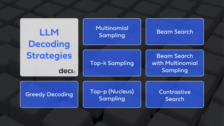
🔍 Overview of LLM Decoding Strategies

Benveniste’s exploration into LLMs focuses on how they predict the next token and generate a stream of tokens relevant to a specific prompt or task.

He details four distinct strategies for text generation, each with pros and cons, and examines how these methods influence the quality of the generated text:

1. 🏹 Greedy Search
2. 🎲 Multinomial Sampling
3. 🔦 Beam Search
4. 🔦 Beam Search w/ Multinomial Sampling
5. 🔄 Contrastive Search

I’ll explore these LLM decoding strategies in depth later in this blog.

🔮 Experiment Vision: Bridging Theory with Practice

There it was, the lightbulb moment.

Why not mesh these generation techniques I’d just wrapped my head around with the IFEval benchmark? What if these text generation strategies could be applied to the models evaluated in the IFEval benchmark? Imagine the insights that could be gleaned from seeing how different methods influence a model’s ability to follow instructions!

It was a perfect blend of theory and practical experimentation, and I was armed with a bunch of Colab Pro+ units at my disposal. It felt like the stars aligning. Perfect for a hands-on experiment, right?

🤖 The Chosen Contenders: DeciLM-7B and Mistral-7B-v0.1

DeciLM-7B and Mistral-7B-v0.1 – these were my guinea pigs.

Each had its own flair, its own promise. The goal was to see how each model responds to the IFEval benchmark under the influence of the different text generation techniques outlined by Benveniste.

⏲️ Against the Clock: GPU Generation Time Tracking

And hey, we’ve been boasting about our model’s speed over Mistral’s.

So I figured an interesting twist to this experiment was monitoring the generation time on the GPU for each model and strategy. This wasn’t just about the quality or fidelity of the generated text; it was also a race against time, measuring the efficiency of each approach in a high-performance computing environment.

A stopwatch in one hand, a magnifying glass in the other – I was ready to see what these models could do, and how quickly they could do it. For the full code, check out this Google Colab notebook.

# @title
%%capture
!pip install huggingface_hub
!pip install transformers
!pip install accelerate
!pip install bitsandbytes
!pip install ninja
!pip install datasets


# for IFEval:
!pip install langdetect nltk absl-py immutabledict

# @title
import os

os.environ['LC_ALL'] = 'en_US.UTF-8'
os.environ['LANG'] = 'en_US.UTF-8'
os.environ['LC_CTYPE'] = 'en_US.UTF-8'

# @title
from huggingface_hub import notebook_login
notebook_login()

# @title
# Standard library imports
import json
import os
from pathlib import Path
from typing import List

# Related third-party imports
import nltk
import torch
from datasets import Dataset, load_dataset
from tqdm import tqdm
from transformers import AutoTokenizer, AutoModelForCausalLM, BitsAndBytesConfig, pipeline

nltk.download('punkt')

# @title
def instantiate_huggingface_model(
    model_name,
    quantization_config=None,
    device_map="auto",
    use_cache=True,
    trust_remote_code=None,
    pad_token=None,
    padding_side="left"
):
    """
    Instantiate a HuggingFace model with optional quantization using the BitsAndBytes library.

    Parameters:
    - model_name (str): The name of the model to load from HuggingFace's model hub.
    - quantization_config (BitsAndBytesConfig, optional): Configuration for model quantization.
      If None, defaults to a pre-defined quantization configuration for 4-bit quantization.
    - device_map (str, optional): Device placement strategy for model layers ('auto' by default).
    - use_cache (bool, optional): Whether to cache model outputs (False by default).
    - trust_remote_code (bool, optional): Whether to trust remote code for custom layers (True by default).
    - pad_token (str, optional): The pad token to be used by the tokenizer. If None, uses the EOS token.
    - padding_side (str, optional): The side on which to pad the sequences ('left' by default).

    Returns:
    - model (PreTrainedModel): The instantiated model ready for inference or fine-tuning.
    - tokenizer (PreTrainedTokenizer): The tokenizer associated with the model.

    The function will throw an exception if model loading fails.
    """

    # If quantization_config is not provided, use the default configuration
    if quantization_config is None:
        quantization_config = BitsAndBytesConfig(
            load_in_4bit=True,
            bnb_4bit_use_double_quant=True,
            bnb_4bit_quant_type="nf4",
            bnb_4bit_compute_dtype=torch.bfloat16
        )

    model = AutoModelForCausalLM.from_pretrained(
        model_name,
        quantization_config=quantization_config,
        device_map=device_map,
        use_cache=use_cache,
        trust_remote_code=trust_remote_code
    )

    tokenizer = AutoTokenizer.from_pretrained(model_name)

    if pad_token is not None:
        tokenizer.pad_token = pad_token
    else:
        tokenizer.pad_token = tokenizer.eos_token
    tokenizer.padding_side = padding_side

    return model, tokenizer

decilm, decilm_tokenizer = instantiate_huggingface_model("Deci/DeciLM-7B-instruct", trust_remote_code=True)

mistral, mistral_tokenizer = instantiate_huggingface_model("mistralai/Mistral-7B-Instruct-v0.1")

deci_generator = pipeline("text-generation",
                          model=decilm,
                          tokenizer=decilm_tokenizer,
                          device_map="auto",
                          max_length=4096,
                          return_full_text=False
)

mistral_generator = pipeline("text-generation",
                          model=mistral,
                          tokenizer=mistral_tokenizer,
                          device_map="auto",
                          max_length=4096,
                          return_full_text=False
)

pipelines = {
    'DeciLM': deci_generator,
    'Mistral': mistral_generator
}

👨🏽‍🎨 LLM Decoding Strategies

⛺️ Baseline

This is an empty dictionary, and it will use the default generation parameters from HuggingFace, except for the temperature setting. Which I will set to a small, near zero value. In my experience with smaller models, I’ve noticed they follow instructions better when temperature is small.

baseline = {}

🏹 Greedy Search Generation

🔧How It Works: Greedy Search selects the most probable next token at each step of the sequence generation. It always chooses the single best option available at the moment without considering the overall sequence. To enable greedy search, you set the parameters num_beams=1 and do_sample=False.

⚖️ Pros and Cons: While this method is simple and fast, it tends to lack creativity and can lead to repetitive or predictable text. This is because it doesn’t look ahead or reconsider past choices.

greedy_config = {
    'num_beams': 1,
    'do_sample': False,
    'temperature': 1e-4
}

🎲 Multinomial Sampling Generation

🔧How It Works: Here, the model chooses words based on a probability distribution, introducing an element of randomness. It samples the next token based on the probability distribution provided by the model, rather than just picking the most probable token. To enable multinomial sampling set do_sample=True and num_beams=1.

It’s like rolling dice for each word, giving the model a chance to generate more diverse and creative text.

⚖️ Pros and Cons: This approach can lead to more varied and interesting outputs but may sometimes generate less coherent or relevant text.

multinomial_config = {
    'num_beams': 1,
    'do_sample': True,
    'temperature': 1e-4
}

🔦 Beam Search Generation

🔧How It Works: Beam Search keeps track of a fixed number of the most probable sequences at each step and expands each of them for the next token. It balances between greedy and exhaustive searches. Beam search is enabled when you specify a value for num_beams (aka number of hypotheses to keep track of) that is bigger than 1.

⚖️ Pros and Cons: This method often leads to more coherent and high-quality text but can be slower and more computationally intensive than greedy search. The quality of the result depends heavily on the size of the “beam” (the number of sequences considered).

beam_search_config = {
    'num_beams': 5,
    'do_sample': False,
    'temperature': 1e-4,
    'early_stopping':True
}

🔦Beam Search w/ 🎲 Multinomial

🔧How It Works: This approach combines Beam Search and Multinomial Sampling, where the Beam Search is applied with a level of randomness in selecting the next tokens. To use this decoding strategy you need to set num_beams to be bigger than 1, and do_sample=True.

⚖️ Pros and Cons: Balances the benefits of Beam Search in generating coherent sequences with the creativity of Multinomial Sampling. But, it’s more complex and computationally demanding.

beam_search_multinomial_config = {
    'num_beams': 5,
    'do_sample': True,
    'temperature': 1e-4,
    'early_stopping':True
}

🔄 Contrastive Search Generation

🔧How It Works: Contrastive Search aims to reduce the typicality of the generated text by contrasting the chosen token with other potential candidates, considering both probability and diversity. The two main parameters that enable and control the behavior of contrastive search are penalty_alpha and top_k. Involves assessing the best tokens and applying penalties to reorder them based on criteria like repetition and diversity. Note, you can read about this method in the orginal 2022 paper, A Contrastive Framework for Neural Text Generation

⚖️ Pros and Cons: While promoting diversity and novelty in responses, this method might sacrifice some degree of relevance or coherence. Requires sophisticated mechanisms to balance between contrastiveness and relevance.

contrastive_search_config = {
    'penalty_alpha': 0.42,
    'top_k': 250,
    'temperature': 1e-4
}

📖 Put all settings in a dictionary

This just makes it easier to iterate over everything.

gen_configs = {
    "baseline":baseline,
    "greedy_search":greedy_config,
    "multinomial_sampling":multinomial_config,
    "beam_search":beam_search_config,
    "beam_search_multinomial":beam_search_multinomial_config,
    "contrastive_search":contrastive_search_config
}

🚀 The Dataset Dilemma: 540+ Rows

We’ve got a dataset here that’s over 540 rows strong. But let’s not get carried away – this is a blog, not a thesis. For simplicity’s sake, we’re narrowing it down.

🔢 Generation Overload: 10 Rounds per Prompt

Each prompt gets the full treatment – 12 generations, each with a different model + config combo.

So, that’s 12 variations for every single prompt.

⏱ The Reality of Local LLMs: It’s a Time-Eater

Anyone who’s dabbled with local LLMs knows this: Text generation takes its sweet time. To keep this post from turning into a marathon, I’m picking 100 prompts at random.

👊 For the Hardcore

Got time and GPUs to burn? Feel free to run the gauntlet with all 540+ prompts.

# @title
dataset = load_dataset("harpreetsahota/Instruction-Following-Evaluation-for-Large-Language-Models", split='train')

dataset = dataset.shuffle(seed=42)
subset = dataset.select(range(100))

# You'll need this as a jsonl file later, so let's save it now
subset.to_json('subset_for_eval.jsonl')

def convert_kwargs_in_jsonl(file_path):
    """
    Modifies a JSONL file by converting 'kwargs' from a JSON-formatted string to a dictionary.

    This adjustment is necessary because the Hugging Face datasets library automatically expands
    schemas, potentially altering the original structure of data with variable schema fields like 'kwargs'.
    Converting 'kwargs' to a dictionary before loading into Hugging Face datasets avoids this issue.

    Parameters:
    - file_path (str): Path to the JSONL file to be modified.

    The function overwrites the original file with the modified data. Ensure to backup the original file
    before running this function.

    Example:
    convert_kwargs_in_jsonl("path/to/jsonl_file.jsonl")
    """
    modified_data = []

    with open(file_path, 'r') as file:
        for line in file:
            line_data = json.loads(line)
            if 'kwargs' in line_data and isinstance(line_data['kwargs'], str):
                line_data['kwargs'] = json.loads(line_data['kwargs'])
            modified_data.append(line_data)

    with open(file_path, 'w') as file:
        for item in modified_data:
            file.write(json.dumps(item) + '\n')

# Replace 'your_file.jsonl' with the path to your JSONL file
convert_kwargs_in_jsonl("/content/subset_for_eval.jsonl")

# @title
SYSTEM_PROMPT_TEMPLATE = """
### System:
You are an AI assistant that follows instructions extremely well. Help as much as you can.
### User:
{instruction}
### Assistant:
"""

def get_prompt_with_template(message: str) -> str:
    return SYSTEM_PROMPT_TEMPLATE.format(instruction=message)

def preprocess_prompt(model_name: str, prompt: str) -> str:
    if model_name == 'DeciLM':
        return get_prompt_with_template(prompt)
    elif model_name == 'Mistral':
        return f"<s>[INST]{prompt}[/INST]"
    else:
        return prompt  # Default case, no special preprocessing

def generate_responses(row, model_name, pipeline, config):
    """
    Generates a response using a specified model with a given generation configuration
    and measures the time taken for generation on the GPU.

    Parameters:
    row (dict): A dictionary representing a row in the dataset.
    model_name (str): The name of the model.
    pipeline (Pipeline): The pipeline object for the model.
    config (dict): The generation configuration.

    Returns:
    dict: Generated text and the time taken for generation.
    """
    # Preprocess prompt based on the model
    processed_prompt = preprocess_prompt(model_name, row['prompt'])

    # Initialize CUDA events for timing
    start_event = torch.cuda.Event(enable_timing=True)
    end_event = torch.cuda.Event(enable_timing=True)

    # Time the generation process
    start_event.record()
    try:
        response = pipeline(processed_prompt, **config)[0]['generated_text']
    except RuntimeError as e:
        response = "Failed Generation"
    end_event.record()

    # Synchronize and calculate time
    torch.cuda.synchronize()
    time_taken = start_event.elapsed_time(end_event) / 1000.0  # Time in seconds
    return {f'{model_name}_response': response, f'{model_name}_time': time_taken}

⏳ Just a heads up, this will take a while

The following took ~14 hours to run.

# Iterate over configurations and models, and generate responses
for config_name, config in gen_configs.items():
    for model_name, model_pipeline in pipelines.items():
        # Prepare new column names
        response_column = f'{model_name}_{config_name}_response'
        time_column = f'{model_name}_{config_name}_time'

        # Initialize lists to store data
        responses, times = [], []

        # Process dataset
        for row in tqdm(subset, desc=f'Processing {model_name} with {config_name}'):
            result = generate_responses(row, model_name, model_pipeline, config)
            responses.append(result[f'{model_name}_response'])
            times.append(result[f'{model_name}_time'])

        # Update the dataset with new columns
        subset = subset.add_column(response_column, responses)
        subset = subset.add_column(time_column, times)

Since the above code will take at least a couple of hours to run, it’s a good idea to run the following cell so that you can push your results to HuggingFace after generation is complete.

subset.push_to_hub("<your-hf-username>/IFEval_Experiments")

If you don’t want to run the code yourself, you can go ahead and download the dataset directly if you wish, just run the following line of code.

data = load_dataset("harpreetsahota/IFEval_Experiments", split="train")

But, I encourage you to run this yourself if you can to independently verify my results.

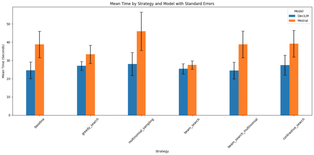
⏱️ Timing Generations

DeciLM consistently proves to be a superior choice, especially when efficiency and speed are the priorities.

DeciLM’s Remarkable Speed: In my comparative analysis across various strategies, DeciLM consistently outperforms Mistral. Its ability to process tasks swiftly is unmatched, making it the go-to option for time-sensitive applications.

Advantages Over Mistral: While Mistral has its merits in handling complex strategies, it falls behind in terms of processing time. DeciLM’s lead in speed is evident and substantial, demonstrating its robustness and superior optimization.

Ideal for a Range of Applications: Whether it’s simple or complex tasks, DeciLM shows remarkable versatility, handling them with greater efficiency than Mistral. This makes DeciLM a more flexible and reliable choice in various scenarios.

The Bottom Line: For anyone looking for a model that delivers quick and efficient results, DeciLM is the undisputed choice. Its performance across different strategies solidifies its position as a top-tier model in the field of AI.

# @title
import pandas as pd
import matplotlib.pyplot as plt
import seaborn as sns

def prepare_average_time_data(dataset, models, strategies):
    """
    Prepare the average time data for plotting.

    Args:
        dataset (Dataset): HuggingFace dataset object.
        models (list): List of model names.
        strategies (list): List of strategies.

    Returns:
        pd.DataFrame: A DataFrame with the average time data.
    """
    # Initialize a dictionary to hold cumulative time and counts for averaging
    time_data = {(model, strategy): {'total_time': 0, 'count': 0}
                 for model in models for strategy in strategies}

    # Process each record in the dataset
    for record in dataset:
        for model in models:
            for strategy in strategies:
                time_column = f"{model}_{strategy}_time"
                if time_column in record and record[time_column] is not None:
                    time_data[(model, strategy)]['total_time'] += record[time_column]
                    time_data[(model, strategy)]['count'] += 1

    # Calculate the average time and prepare data for DataFrame
    data_for_df = []
    for (model, strategy), time_info in time_data.items():
        if time_info['count'] > 0:
            avg_time = time_info['total_time'] / time_info['count']
            data_for_df.append({'Model': model, 'Strategy': strategy, 'Average Time': avg_time})

    return pd.DataFrame(data_for_df)

def plot_average_time_by_strategy(df):
    """
    Plots the average time by strategy for different models.

    Parameters:
    df (DataFrame): A pandas DataFrame containing the columns 'Model', 'Strategy', and 'Average Time'.
    """
    plt.figure(figsize=(12, 6))
    sns.barplot(x='Strategy', y='Average Time', hue='Model', data=df, palette=['blue', 'orange'])
    plt.title('Average Time by Strategy and Model')
    plt.xticks(rotation=45)
    plt.ylabel('Average Time (Seconds)')
    plt.xlabel('Strategy')
    plt.legend(title='Model')
    plt.tight_layout()
    plt.show()

models = ['DeciLM', 'Mistral']
strategies = ['baseline', 'greedy_search', 'multinomial_sampling', 'beam_search', 'beam_search_multinomial', 'contrastive_search']

df_avg_time = prepare_average_time_data(subset, models, strategies)

plot_average_time_by_strategy(df_avg_time)

👨🏾‍🍳 Prepare for Evaluation with IFEval

In order to run IFEval we’ll need to prepare our environment and datasets.

Here’s what needs to be done:

• Clone the repo and install dependencies
• Format data: Save each generation + strategy combo from the dataset we created as a jsonl file with two entries: prompt and response

Clone the repo

The IFEval code is in the Google Research repo, which is massive. The below code will download the entire repo but only extract the IFEval code.

%%bash
curl -L https://github.com/google-research/google-research/archive/master.zip -o google-research-master.zip
unzip google-research-master.zip "google-research-master/instruction_following_eval/*"

👩🏿‍🔧 Install dependencies

!pip install absl-py
!pip install -r /content/google-research-master/instruction_following_eval/requirements.txt
!mkdir /content/output

🔷 Format Data

def save_as_jsonl(dataset: Dataset, prompt_column: str, response_column: str, output_dir: Path) -> None:
    """
    Saves specific columns of a Hugging Face dataset as JSONL files.

    Args:
        dataset (Dataset): The Hugging Face dataset to process.
        prompt_column (str): The name of the column in the dataset that contains the prompts.
        response_column (str): The name of the column in the dataset that contains the responses.
        output_dir (Path): The directory where the JSONL files will be saved.

    Returns:
        None
    """
    output_file = output_dir / f'{response_column}.jsonl'
    with open(output_file, 'w') as f:
        for example in dataset:  # Replace 'train' with the appropriate dataset split
            json_object = {
                "prompt": example[prompt_column],
                "response": example[response_column]
            }
            f.write(json.dumps(json_object) + '\n')

# Define your prompt and response columns
prompt_column = 'prompt'

response_columns = ['DeciLM_baseline_response',
                    'Mistral_baseline_response',
                    'DeciLM_greedy_search_response',
                    'Mistral_greedy_search_response',
                    'DeciLM_multinomial_sampling_response',
                    'Mistral_multinomial_sampling_response',
                    'DeciLM_beam_search_response',
                    'Mistral_beam_search_response',
                    'DeciLM_beam_search_multinomial_response',
                    'Mistral_beam_search_multinomial_response',
                    'DeciLM_contrastive_search_response',
                    'Mistral_contrastive_search_response']

output_dir = Path('/content/google-research-master/instruction_following_eval/data')

for response_column in response_columns:
    save_as_jsonl(subset, prompt_column, response_column, output_dir)

🛠 IFEval in Action

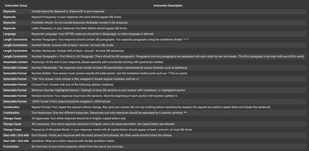
The implementation involved crafting 25 verifiable instructions into 541 diverse prompts, a process that was both meticulous and rigorous:

• Generating base prompts: This foundational step involved creating the initial set of prompts that would be further refined.
• Using AI for initial vetting: At this stage, AI tools were employed to evaluate the prompts, ensuring they met the basic criteria for verifiability and clarity.
• Adding variety in phrasing: To ensure a comprehensive evaluation, each prompt was rephrased to increase the diversity of its presentation, avoiding monotonous or repetitive phrasing.
• A final manual review: This crucial step involved a thorough manual inspection of the rephrased prompts to guarantee their quality, relevance, and alignment with the intended instructional goals.

The table below describes the 25 verifiable instructions, and their descriptions.

Example prompt, instruction, and generations

You’ll notice the complete prompt that should be provided as input to the model, and a list of instructions and key word arguments that the framework uses to assess adherence to the prompt.

You can also see an example of the completion from each models baseline configuration.

subset[42]['prompt'], subset[42]['instruction_id_list'], subset[42]['kwargs']

('Can you give me an example for a journal entry about stress management? Tell me how you come up with the example. Your entire response should contain less than 6 sentences.',
 ['length_constraints:number_sentences'],
 '[{"relation": "less than", "num_sentences": 6}]')

print(subset[42]['DeciLM_baseline_response']),

Result:

Sure, here's an example of a journal entry about stress management:

"Today, I experienced a lot of stress due to a heavy workload and personal issues. To manage my stress, I decided to take a break and go for a walk. As I walked, I focused on my breath and the beauty of nature around me. This helped me feel more relaxed and recharged, allowing me to approach my tasks with a clearer mind."

I came up with this example by thinking about common stressors and how people might manage them. I then used my own experience to create a relatable and helpful entry.

print(subset[42]['Mistral_baseline_response'])

Result:

 Example: "Today, I practiced stress management by taking a break from technology and spending time in nature. I went for a walk in the park and listened to the sound of the birds and the rustling of the leaves. This helped me to clear my mind and reduce feelings of anxiety and stress."

I came up with this example by reflecting on my own experiences with stress management. I know that taking a break from technology and spending time in nature can be helpful in reducing stress levels. So, I decided to write about a specific instance where I practiced this technique and the positive effects it had on me.

How does IFEval work?

This evaluation framework is designed to comprehensively test and compare LLMs based on their ability to understand and follow instructions. It combines strict and loose accuracy assessments at both the prompt and instruction levels, supported by a robust testing system to ensure the accuracy and reliability of the evaluation process.

1. Preparation: The system sets up instructions using the instruction framework and loads input data.
2. Evaluation: The evaluation_main.py script processes these inputs and compares the system’s responses against the expected outcomes defined by the instructions.
3. Result Analysis: The system generates results that detail how well the instructions were followed, under different evaluation criteria (strict vs. loose).
4. Testing and Validation: Test scripts are used throughout to ensure the integrity of the instruction framework and the reliability of the evaluation process.

🏃🏽‍♂️💨 Run Evaluation

I appreciate its objective approach to evaluating language models.

Unlike other methods that might require subjective interpretation or additional language models for evaluation, IFEval offers a clear-cut, binary system: the model either follows the given instruction, or it doesn’t. This simplicity is invaluable, especially when running on CPU without the need for high-powered resources. Such a straightforward evaluation is a vital sanity check in comparing language models, ensuring they meet specific criteria crucial in high-stakes scenarios.

This objectivity in assessment provides a reliable baseline for measuring a model’s instruction-following capabilities, an essential factor in its practical application.

import sys
sys.path.append('/content/google-research-master/instruction_following_eval')

%cd /content/google-research-master

log_file = "/content/output/all_responses_log.txt"  # Single log file for all responses
os.makedirs("/content/output", exist_ok=True)

for response_column in response_columns:
    response_file = f"/content/google-research-master/instruction_following_eval/data/{response_column}.jsonl"
    output_dir = f"/content/output/{response_column}"

    # Create the output directory if it doesn't exist
    os.makedirs(output_dir, exist_ok=True)

    # Run the script for each response file and append output to the log file
    !python -m instruction_following_eval.evaluation_main \
      --input_data=/content/subset_for_eval.jsonl \
      --input_response_data={response_file} \
      --output_dir={output_dir} &>> {log_file}

    print(f"Completed evaluation for {response_column}")

# Print a message when all processing is complete
print(f"All evaluations complete. Check the log file: {log_file} for details.")

# @title

import re
import pandas as pd
def parse_log(file_path):
    """
    Parses the log file to extract baseline response names and their associated
    accuracy scores under both strict and loose evaluation regimes.

    Parameters:
    file_path (str): Path to the log file.

    Returns:
    dict: A dictionary with the results for strict and loose
    """
    # Regular expression to match the relevant lines in the log data
    pattern = r"/content/output/(?P<response>[\w_]+)/eval_results_(?P<type>\w+).jsonl Accuracy Scores:\n" \
              r"prompt-level: (?P<prompt_level>[\d.]+)\n" \
              r"instruction-level: (?P<instruction_level>[\d.]+)\n"

    # Dictionary to store the parsed data
    results = {}

    # Read the log file
    with open(file_path, 'r') as file:
        log_data = file.read()

        # Find all matches and process them
        for match in re.finditer(pattern, log_data, re.MULTILINE):
            response = match.group("response")
            eval_type = f"eval_results_{match.group('type')}"
            prompt_level = float(match.group("prompt_level"))
            instruction_level = float(match.group("instruction_level"))

            # Initialize the response dictionary if not already present
            if response not in results:
                results[response] = {}
            # Store the scores in the corresponding dictionary
            results[response][eval_type] = {
                "prompt-level": prompt_level,
                "instruction-level": instruction_level
            }

    return results

parsed_log = parse_log("/content/output/all_responses_log.txt")

# Create a list of dictionaries for DataFrame construction
data_for_df = []
for response_name, response_data in parsed_log.items():
    # Split the response_name to separate the model and the strategy
    parts = response_name.split('_')
    model_name = parts[0]
    strategy = '_'.join(parts[1:-1])  # Join all parts except the first and last

    # Now create a row for each eval_type
    for eval_type, scores in response_data.items():
        row = {
            'Model': model_name,
            'Strategy': strategy,
            'Evaluation Type': eval_type.split('_')[-1],  # Get 'strict' or 'loose'
            'Prompt Level': scores['prompt-level'],
            'Instruction Level': scores['instruction-level']
        }
        data_for_df.append(row)

# Create the DataFrame
df = pd.DataFrame(data_for_df)

# @title
import matplotlib.pyplot as plt
import pandas as pd

def get_strategy_data(df, strategy):
    """
    Filter the DataFrame for a specific strategy.

    Args:
        df (pd.DataFrame): The DataFrame to filter.
        strategy (str): The strategy to filter by.

    Returns:
        pd.DataFrame: Filtered DataFrame.
    """
    return df[df['Strategy'] == strategy]

def plot_model_bars(ax, strategy_data, model_colors, bar_positions, strategy_index):
    """
    Plot bars for each model in the given strategy data.

    Args:
        ax (matplotlib.axes.Axes): The axis to plot on.
        strategy_data (pd.DataFrame): Data for the specific strategy.
        model_colors (dict): A dictionary mapping models to colors.
        bar_positions (list): Positions for each bar in the plot.
        strategy_index (int): Index of the current strategy.

    Returns:
        None
    """
    for j, (model, color) in enumerate(model_colors.items()):
        prompt_level = strategy_data[strategy_data['Model'] == model]['Prompt Level'].values
        if prompt_level.size > 0:
            ax.bar(bar_positions[j], prompt_level[0], color=color, width=0.4, label=model if strategy_index == 0 else "")

def plot_evaluation(df, evaluation_type, model_colors, ax, strategies, column_to_plot):
    """
    Plot the evaluation data as a bar chart for a specified column.

    Args:
        df (pd.DataFrame): The DataFrame containing evaluation data.
        evaluation_type (str): The type of evaluation ('strict' or 'loose').
        model_colors (dict): A dictionary mapping models to colors.
        ax (matplotlib.axes.Axes): The matplotlib axis to plot on.
        strategies (list): A list of strategies to evaluate.
        column_to_plot (str): The column name to plot.

    Returns:
        None
    """
    for i, strategy in enumerate(strategies):
        strategy_data = df[df['Strategy'] == strategy]
        bar_positions = [i - 0.2, i + 0.2]

        for j, (model, color) in enumerate(model_colors.items()):
            values = strategy_data[strategy_data['Model'] == model][column_to_plot].values
            if values.size > 0:
                ax.bar(bar_positions[j], values[0], color=color, width=0.4, label=model if i == 0 else "")

    ax.set_xticks(range(len(strategies)))
    ax.set_xticklabels(strategies, rotation=45, ha='right')
    ax.set_ylabel(column_to_plot.replace('_', ' ').title())
    ax.set_title(f"{evaluation_type.capitalize()} Evaluation: {column_to_plot.replace('_', ' ').title()}")

    if evaluation_type == 'strict':
        handles, labels = ax.get_legend_handles_labels()
        ax.legend(handles, labels, loc='best')

def plot_strict_and_loose(df, model_colors, column_to_plot):
    """
    Set up and plot for strict and loose evaluations for a specified column.

    Args:
        df (pd.DataFrame): The DataFrame containing the evaluation data.
        model_colors (dict): A dictionary mapping models to colors.
        column_to_plot (str): The column name to plot.

    Returns:
        None
    """
    df_strict = df[df['Evaluation Type'] == 'strict']
    df_loose = df[df['Evaluation Type'] == 'loose']
    strategies = sorted(df['Strategy'].unique())

    fig, axs = plt.subplots(1, 2, figsize=(14, 7), sharey=True)
    plot_evaluation(df_strict, 'strict', model_colors, axs[0], strategies, column_to_plot)
    plot_evaluation(df_loose, 'loose', model_colors, axs[1], strategies, column_to_plot)

    plt.tight_layout()
    plt.show()

# Example usage
model_colors = {'DeciLM': 'blue', 'Mistral': 'orange'}

📏 Clear Metrics for Evaluation

IFEval introduces two key metrics for evaluating the adherence of large language models (LLMs) to instructions:

1. ✅ Strict Accuracy: This metric is a straightforward assessment: did the LLM follow the instructions exactly as stated? It’s a binary evaluation—either the instruction was followed (True) or it wasn’t (False).
2. 🔄 Loose Accuracy: Recognizing the complexity and potential nuances in language, this more lenient metric allows for transformations in the responses. It aims to reduce false negatives by accounting for variations in how instructions might be correctly but differently executed.

🔍 Bringing It All Together

The evaluation results in four distinct accuracy scores, combining strict and loose assessments at both the prompt and instruction levels:

1. 🎯 Prompt-level strict-accuracy
2. 📏 Instruction-level strict-accuracy
3. 🌐 Prompt-level loose-accuracy
4. 🔍 Instruction-level loose-accuracy

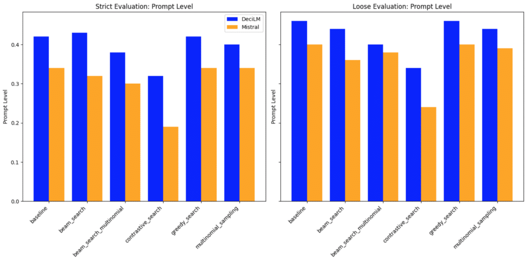
Prompt level evaluation: comparing the models with different LLM decoding strategies

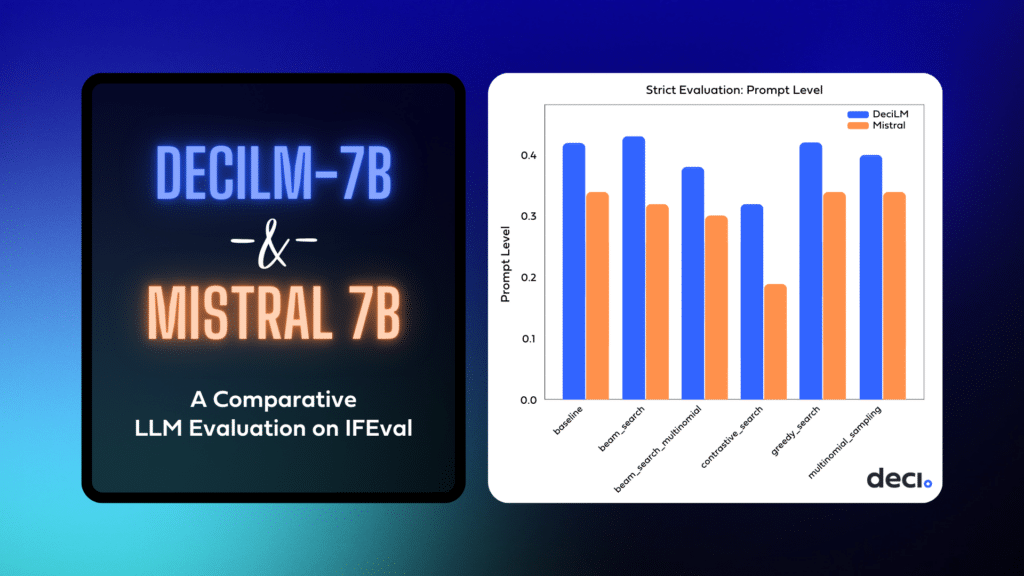
🎯 Prompt-level strict-accuracy

This metric calculates the percentage of prompts in which all verifiable instructions within each prompt are followed. Essentially, it assesses the model’s ability to adhere to every instruction within a single prompt.

• DeciLM consistently outperforms Mistral in strict accuracy across all strategies. Its highest strict accuracy is observed with the ‘beam_search’ strategy (0.43), indicating its superior capability in following instructions precisely.
• Mistral shows lower strict accuracy, with its highest being 0.34 under the ‘baseline’ and ‘greedy_search’ strategies. This suggests a relative weakness in adhering to instructions exactly as stated compared to DeciLM.

🌐 Prompt-level loose-accuracy

This is the prompt-level accuracy computed with a loose criterion. The ‘loose’ criterion involves more lenient standards for following instructions, allowing for variations in the responses that still capture the essence of the instructions.

• DeciLM also leads in loose accuracy, demonstrating a better understanding of the essence of instructions. Its highest score is 0.46, achieved with both ‘baseline’ and ‘greedy_search’ LLM decoding strategies.
• Mistral, while trailing behind DeciLM, shows its best performance in loose accuracy with the ‘baseline’ and ‘greedy_search’ LLM decoding strategies (0.40). This indicates a reasonable ability to capture the intent of instructions, though not as effectively as DeciLM.

DeciLM clearly outperforms Mistral in both strict and loose accuracy metrics at the prompt level, regardless of the strategy used. This suggests that DeciLM is better equipped to understand and adhere to instructions in a variety of contexts. Mistral, while showing reasonable capability, particularly in loose accuracy, falls behind in strictly adhering to instructions, indicating potential areas for improvement.

Overall, DeciLM demonstrates a superior balance in understanding the literal and nuanced aspects of instructions, making it the more effective model for tasks requiring both precision and adaptability in language understanding.

# column_to_plot =   # Specify the column you want to plot
plot_strict_and_loose(df, model_colors, column_to_plot='Prompt Level')

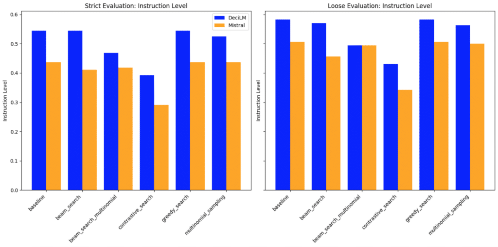
Instruction level eval: comparing the models with different LLM decoding strategies

📏 Instruction-level strict-accuracy

This metric measures the percentage of individual verifiable instructions that are followed, regardless of the prompt they appear in. It focuses on the model’s consistency in following each type of instruction across different prompts.

• DeciLM’s scores are higher, indicating a better ability to adhere to instructions exactly as stated.
• Mistral’s lower scores suggest a need for improvement in strict adherence to instructions.

🔍 Instruction-level loose-accuracy

Similar to prompt-level loose accuracy, this metric is computed at the instruction level with a loose criterion. It evaluates how well the model follows each instruction across different prompts, with some leniency in how strictly the instructions need to be adhered to.

• DeciLM again leads, showing its capability to interpret instructions with some flexibility.
• Mistral performs better in loose accuracy than strict, but still trails behind DeciLM.

DeciLM demonstrates stronger performance in instruction adherence at the instruction level, both strictly and loosely, across all evaluated strategies. Mistral, while showing some capability, especially in loose accuracy, needs improvements to match the performance of DeciLM.

The choice of strategy significantly affects the models’ performance, highlighting the importance of strategy selection in model deployment for specific tasks.

plot_strict_and_loose(df, model_colors, column_to_plot='Instruction Level')

🚀 Wrapping Up: A Wild Ride Through LLM Decoding Strategies and Evaluation

We’re at the end of this wild, caffeinated sprint through the land of LLM evals. And what a ride it’s been! Big shout out to the authors whose genius lit the fuse for this firecracker of a project. Your work more than sparked my curiosity; it set off a full-blown fireworks show in my brain!

Juggling the intricacies of LLM evaluation and LLM decoding strategies has been both challenging and immensely enjoyable.

In my opinion the IFEval framework is a gem and has rightly earned its place in my evals toolkit. It offers a fresh perspective on how we assess instruction-following in language models. To my fellow AI enthusiasts, I hope my explorations shed some light on this framework’s potential. For deeper dives and lively discussions, I’m just a message away – let’s keep the conversation going in the Deep Learning Daily Discord community here.

Embarking on this project, I was stepping into the unknown. Starting this project, I had no clue what to expect. Mistral v0.1 was strutting its stuff on the leaderboard, but then – plot twist! – DeciLM swooped in like a superhero, nailing task after task. Didn’t see that coming!

As we look ahead, the comparison with Mistral v0.2 is the next frontier.

I’m throwing down the gauntlet to the community – take my work, build on it, challenge it. Independent exploration by others in the community is not just welcome, it’s essential for validating and enriching our collective understanding.

Curious to dive deeper into the technical intricacies of DeciLM-7B? Explore our comprehensive technical blog for a detailed analysis and insights into its advanced capabilities.

Discover Deci’s LLMs and GenAI Development Platform

In addition to DeciLM-7B, Deci offers a suite of fine-tunable high performance LLMs, available through our GenAI Development Platform. Designed to balance quality, speed, and cost-effectiveness, our models are complemented by flexible deployment options. Customers can access them through our platform’s API or opt for deployment on their own infrastructure, whether through a Virtual Private Cloud (VPC) or directly within their data centers.

If you’re interested in exploring our LLMs firsthand, we encourage you to sign up for a free trial of our API.

For those curious about our VPC and on-premises deployment options, we encourage you to book a 1:1 session with our experts.