How to Train YOLO-NAS with SuperGradients: A Step-by-Step Guide

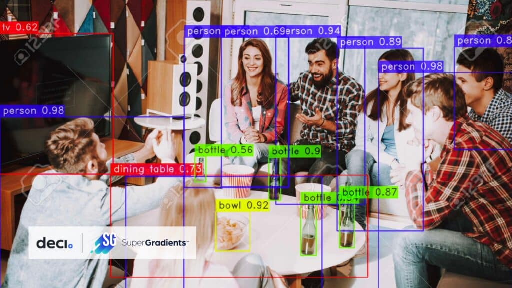
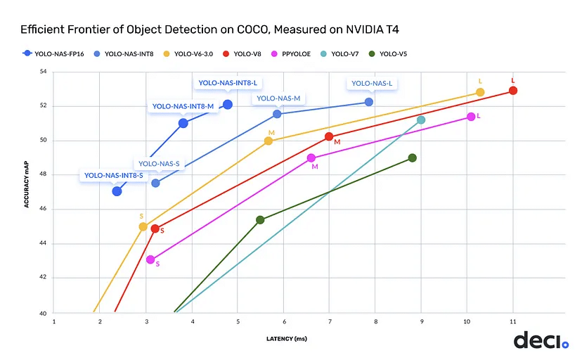
YOLO-NAS marks a significant advancement in object detection, offering improvements over previous models like YOLOv5 through YOLOv8. This model is engineered for higher accuracy and speed, addressing challenges such as limited quantization support and the balance between accuracy and latency. Its training on comprehensive datasets like COCO and Objects365 equips YOLO-NAS for effective deployment across a range of production scenarios. The model is available in three variants – yolo_nas_s, yolo_nas_m, and yolo_nas_l, each tailored to different performance and resource requirements.

SuperGradients, a PyTorch-based training library, complements YOLO-NAS by providing tools for various computer vision tasks, including detection, segmentation, and pose estimation. With an array of nearly 40 pre-trained models, the library facilitates the integration and optimization of sophisticated models like YOLO-NAS for specific use cases.

This blog is centered on effectively training YOLO-NAS on custom datasets using SuperGradients. Aimed at computer vision practitioners and data scientists, it offers a direct, practical guide for applying YOLO-NAS to your specific dataset challenges, demonstrating the practical utility of this combination in real-world applications.

🏋🏽 Setting Up the Trainer in SuperGradients

The heart of your training process in SuperGradients is the Trainer. It handles training, evaluation, and checkpoint management. Begin by defining two key arguments:

1. ckpt_root_dir: The directory for saving results from all experiments – where all your training results will be stored.
2. experiment_name: A designated name under which checkpoints, logs, and tensorboards are stored.
   
   

from super_gradients.training import Trainer

CHECKPOINT_DIR = 'checkpoints'
trainer = Trainer(experiment_name='my_custom_yolonas_run', ckpt_root_dir=CHECKPOINT_DIR)

🔍 Dataset Selection, Loading, Transformations, and Visualization

Choose Your Dataset

SuperGradients is fully compatible with PyTorch datasets. There are several well-known datasets for object detection, including COCO and Pascal. 

For this example you’ll use the the U.S. Coins Dataset from RoboFlow with the dataset in YOLOv5 format.

Import the Dataset 

Utilize the Roboflow library to import the dataset:

from roboflow import Roboflow

rf = Roboflow(api_key="your_api_key")
project = rf.workspace("your_workspace").project("u.s.-coins-dataset")
dataset = project.version(5).download("yolov5")

Configure the Dataset Parameters

When preparing your dataset for training with SuperGradients, it’s crucial to define and organize your dataset parameters effectively. This involves creating a dictionary in Python that outlines key elements of your dataset’s structure:

• Parent Directory Path: Specify the path to the main directory where your dataset resides. This is your dataset’s root folder, containing all the data files.
• Child Directories for Dataset Segments: Clearly define the names of the subdirectories for different parts of your dataset:
  • Training Data: Include paths to both the images and labels for training.
  • Validation Data: Similarly, specify paths for validation images and labels.
  • Testing Data (optional): If you have a separate testing set, provide paths for the test images and labels.
• Class Names: List out the names of the classes your model will be detecting. 
  
  

Here’s a concise way to encapsulate this information in your code:

dataset_params = {
   'data_dir':'/content/U.S.-Coins-Dataset---A.Tatham-5',
   'train_images_dir':'train/images',
   'train_labels_dir':'train/labels',
   'val_images_dir':'valid/images',
   'val_labels_dir':'valid/labels',
   'test_images_dir':'test/images',
   'test_labels_dir':'test/labels',
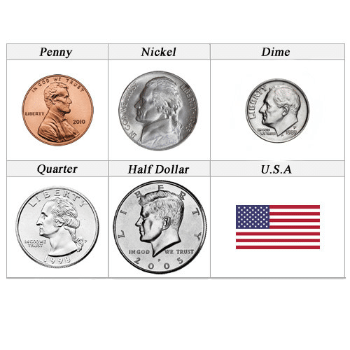
   'classes': ['Dime', 'Nickel', 'Penny', 'Quarter']}

Set up Dataloaders

SuperGradients provides ready-to-use dataloaders for the datasets it supports. Import required modules for SuperGradients dataloaders.

from super_gradients.training import dataloaders
from super_gradients.training.dataloaders.dataloaders import coco_detection_yolo_format_train, coco_detection_yolo_format_val

Create data loaders for training, validation, and testing sets with specified batch size and number of workers. Below we use batch_size=16 and num_workers=2. Note that for training and testing data we use coco_detection_yolo_format_val to instantiate the dataloader.

from IPython.display import clear_output


train_data = coco_detection_yolo_format_train(
   dataset_params={
       'data_dir': dataset_params['data_dir'],
       'images_dir': dataset_params['train_images_dir'],
       'labels_dir': dataset_params['train_labels_dir'],
       'classes': dataset_params['classes']
   },
   dataloader_params={
       'batch_size':16,
       'num_workers':2
   }
)


val_data = coco_detection_yolo_format_val(
   dataset_params={
       'data_dir': dataset_params['data_dir'],
       'images_dir': dataset_params['val_images_dir'],
       'labels_dir': dataset_params['val_labels_dir'],
       'classes': dataset_params['classes']
   },
   dataloader_params={
       'batch_size':16,
       'num_workers':2
   }
)


test_data = coco_detection_yolo_format_val(
   dataset_params={
       'data_dir': dataset_params['data_dir'],
       'images_dir': dataset_params['test_images_dir'],
       'labels_dir': dataset_params['test_labels_dir'],
       'classes': dataset_params['classes']
   },
   dataloader_params={
       'batch_size':16,
       'num_workers':2
   }
)


clear_output()

Handle Annotations and Transforms

• The dataloaders will manage annotations and can print warnings for non-conforming formats.
• SuperGradients automatically adds transforms to the dataset, which you can customize or extend as needed.
  
  

Inspect and Modify Transforms

Examine and modify dataset transforms if necessary:

train_data.dataset.transforms
# Modify specific transform parameters as needed

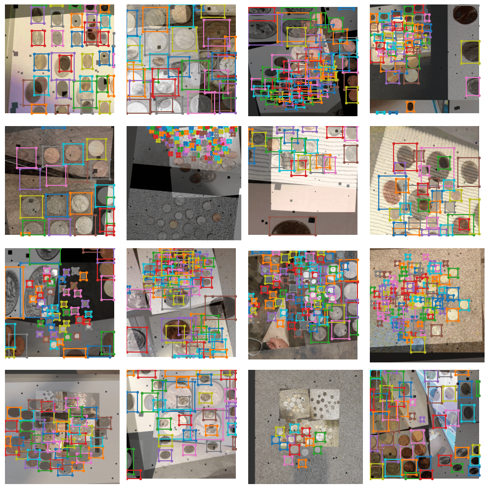
Visualize Augmented Data

You can plot a batch of training data with their augmentations to see what they look like: 

train_data.dataset.plot()

👩🏽‍🦳 Model Instantiation for Fine-Tuning

Choose the YOLO-NAS variant (e.g., yolo_nas_l) and instantiate the model, specifying the number of classes based on your dataset.

from super_gradients.training import models

model = models.get('yolo_nas_l', num_classes=len(dataset_params['classes']), pretrained_weights="coco")

📊 Training Parameters and Metrics

In configuring your training with SuperGradients, the definition of training parameters plays a crucial role. These settings not only dictate your training process but also significantly impact the performance of your model. Here’s a concise overview of the essential parameters and some advanced features you should consider:

Essential Training Parameters

• max_epochs: Sets the maximum number of training cycles.
• loss: Choose a suitable loss function for your model and dataset.
• optimizer: Opt for an optimizer (e.g., Adam, AdamW, SGD) and customize it if necessary through optimizer_params.
• train_metrics_list/valid_metrics_list: Specify metrics for evaluating training and validation performance. These are implemented as Torchmetric objects.
• metric_to_watch: Select a primary metric to determine checkpoint saving.
  
  

Advanced Features and Integrations

• Monitoring Tools: Utilize integrations with Tensorboard, Weights and Biases, or ClearML for tracking training progress. Custom integrations can be achieved using BaseSGLogger.
• Training Enhancements: SuperGradients offers features like Exponential Moving Average, Zero Weight Decay on Bias and Batch Normalization, Weight Averaging, Batch Accumulation, and Precise BatchNorm for optimized training.
• Custom Metrics: SuperGradients supports the creation of custom metrics for specialized needs.
  
  

Loss and Detection Metrics Setup

For functions like PPYoloELoss and DetectionMetrics_050, ensure you specify the number of classes in your dataset correctly to align loss calculations and metrics evaluation with your dataset’s specifics.

from super_gradients.training.losses import PPYoloELoss
from super_gradients.training.metrics import DetectionMetrics_050
from super_gradients.training.models.detection_models.pp_yolo_e import PPYoloEPostPredictionCallback


train_params = {
   # ENABLING SILENT MODE
   'silent_mode': True,
   "average_best_models":True,
   "warmup_mode": "linear_epoch_step",
   "warmup_initial_lr": 1e-6,
   "lr_warmup_epochs": 3,
   "initial_lr": 5e-4,
   "lr_mode": "cosine",
   "cosine_final_lr_ratio": 0.1,
   "optimizer": "Adam",
   "optimizer_params": {"weight_decay": 0.0001},
   "zero_weight_decay_on_bias_and_bn": True,
   "ema": True,
   "ema_params": {"decay": 0.9, "decay_type": "threshold"},
   # ONLY TRAINING FOR 10 EPOCHS FOR THIS EXAMPLE NOTEBOOK
   "max_epochs": 10,
   "mixed_precision": True,
   "loss": PPYoloELoss(
       use_static_assigner=False,
       # NOTE: num_classes needs to be defined here
       num_classes=len(dataset_params['classes']),
       reg_max=16
   ),
   "valid_metrics_list": [
       DetectionMetrics_050(
           score_thres=0.1,
           top_k_predictions=300,
           # NOTE: num_classes needs to be defined here
           num_cls=len(dataset_params['classes']),
           normalize_targets=True,
           post_prediction_callback=PPYoloEPostPredictionCallback(
               score_threshold=0.01,
               nms_top_k=1000,
               max_predictions=300,
               nms_threshold=0.7
           )
       )
   ],
   "metric_to_watch": '[email protected]'
}

🦾 Commencing the Training

You’ve covered a lot of ground so far:

✅ Instantiated the trainer

✅ Defined your dataset parameters and dataloaders

✅ Instantiated a model

✅ Set up your training parameters

Now it’s time to start the training process with the configured model, training parameters, and data loaders.

It’s as easy as…

trainer.train(model=model, training_params=train_params, train_loader=train_data, valid_loader=val_data)

🏆 Retrieving the Best Trained Model

After completing the training process, the next crucial step is to obtain the model that has performed the best during your training sessions. In SuperGradients, this involves selecting the most effective set of weights from your training runs. You have a couple of options based on your training strategy and goals:

Using Checkpoint Averaging

SuperGradients implements checkpoint averaging. This approach combines weights from various epochs to achieve a more balanced and potentially robust model. It averages out the fluctuations and inconsistencies that might occur in different training stages. The code for retrieving a model with averaged weights would look something like this:

from super_gradients.training import models

# Path to the averaged checkpoint
averaged_checkpoint_path = 'checkpoints/my_first_yolonas_run/average_model.pth'

# Retrieve the model with averaged weights
best_model = models.get('yolo_nas_l', 
                        num_classes=len(dataset_params['classes']),
                        checkpoint_path=averaged_checkpoint_path)

Choosing Best or Last Weights

Alternatively, you might prefer using the absolute best weights from a single epoch or the weights from the last epoch of training. The choice between these depends on whether you prioritize the peak performance achieved at any point (best weights) or the final state of the model after the last training epoch (last weights).

Here’s how you can load the model with these weights:

Best Weights:

best_weights_path = 'checkpoints/my_first_yolonas_run/ckpt_best.pth'
best_model = models.get('yolo_nas_l', 
                        num_classes=len(dataset_params['classes']),
                        checkpoint_path=best_weights_path)

Last Weights:

last_weights_path = 'checkpoints/my_first_yolonas_run/ckpt_latest.pth'
last_model = models.get('yolo_nas_l', 
                        num_classes=len(dataset_params['classes']),
                        checkpoint_path=last_weights_path)

Each of these methods has its own advantages, and the choice largely depends on your specific project requirements and the nature of your training data. Experimenting with both can provide insights into what works best for your particular use case.

🧐 Model Evaluation on Test Data

Evaluate your model on the test dataset to understand its performance in real-world scenarios.

trainer.test(model=best_model,
           test_loader=test_data,
           test_metrics_list=DetectionMetrics_050(score_thres=0.1,
                                                  top_k_predictions=300,
                                                  num_cls=len(dataset_params['classes']),
                                                  normalize_targets=True,
                                                  post_prediction_callback=PPYoloEPostPredictionCallback(score_threshold=0.01,
                                                                                                         nms_top_k=1000,
                                                                                                         max_predictions=300,                                                                             
                                                                                                         nms_threshold=0.7)
                                                 ))

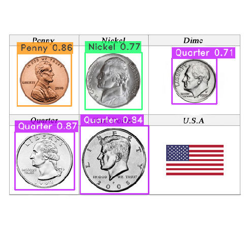
The next line of code will perform prediction on the linked image. Note, that we didn’t have a class for the half-dollar coin. So it will likely get classified as something else.

img_url = 'https://www.mynumi.net/media/catalog/product/cache/2/image/9df78eab33525d08d6e5fb8d27136e95/s/e/serietta_usa_2_1/www.mynumi.net-USASE5AD160-31.jpg'
best_model.predict(img_url).show()

The results aren’t too bad after just a few epochs!

A Glimpse into Advanced Optimization: PTQ and QAT in SuperGradients

Now that you know how to train YOLO-NAS with SuperGradients, it’s worth briefly touching upon two advanced optimization techniques available in this versatile library: Post Training Quantization (PTQ) and Quantization Aware Training (QAT).

What Are PTQ and QAT?

• Post Training Quantization (PTQ): This technique involves optimizing the model after training by reducing the precision of weights and activations, which can lead to smaller model sizes and faster inference times.
• Quantization Aware Training (QAT): QAT integrates quantization directly into the training process, helping the model adapt to reduced precision. This method is often adopted to compensate for the degradation in accuracy of the quantized model. When done right, it sometimes results in accuracy surpassing that of the orginal, unquantized model. 
  
  

Why Consider These Techniques?

Incorporating PTQ or QAT can significantly boost your model’s efficiency, especially for deployment in environments with limited computational resources. These methods are part of the cutting-edge practices in machine learning, offering a way to enhance your model’s deployment readiness without a major trade-off in accuracy.

Exploring Further

While PTQ and QAT are advanced topics that extend beyond the basics of training YOLO-NAS, they represent the frontier of model optimization and deployment strategies. For those interested in delving deeper into these areas, SuperGradients provides the tools and documentation to explore these techniques further.

Conclusion 

To sum up, training YOLO-NAS using SuperGradients equips you with advanced tools for object detection, blending top-tier model performance with comprehensive training capabilities. As you apply these insights to your projects, keep exploring and refining your approach to stay at the forefront of this rapidly evolving field. This guide is just the beginning of what you can achieve in the realm of computer vision. Happy modeling!

YOLO-NAS is just one part of Deci’s extensive range of foundation models. Within this collection, you’ll find DeciSegs, the SOTA  hyper-performant semantic segmentation models and the YOLO-NAS Pose models, designed for hyper-efficient pose estimation. Each family within Deci’s foundation models is meticulously crafted using the AutoNAC engine. It is tailored to excel in specific computer vision tasks and optimized for given hardware and dataset characteristics.

Upon choosing a foundation or custom model, you can train or fine-tune it using your own data via SuperGradients. To further boost your model’s efficiency and inference speed, Deci’s Infery SDK is an invaluable tool.

Discover more about Infery and using Deci’s foundation models for commercial applications, by booking a demo with us.