
Defining Distribution of Bounding Box Areas
Distribution of Bounding Box Areas refers to the distribution of the areas of bounding boxes, calculated as a percentage of the total image area. This can be analyzed for each class individually, or collectively across all classes, providing insights into the variety of object sizes present in your dataset.
Understanding the distribution of bounding box areas is key, as it can reveal important information about our dataset that may impact our model’s performance. It’s an invaluable tool for identifying variations and trends in object sizes, both within and across classes.
The Importance of the Distribution of Bounding Box Areas
Analyzing the distribution of bounding box areas of your dataset highlights any gaps in object size between the training and validation splits, which may harm model performance.
Additionally, if there are too many very small objects, it may indicate that you are downsizing your original image to a scale that is inappropriate for your objects.
Calculating Distribution of Bounding Box Areas
To calculate the distribution of bounding box area, iterate over all the images in your dataset.
For each image, calculate the area of each bounding box as a percentage of the total image area. This is done by dividing the bounding box’s area by the image’s area and multiplying by 100. Do this separately for the training and validation sets.
The results are then aggregated and visualized using a violin plot, which shows the distribution of object areas for each class. This allows you to compare the object size characteristics of your training set to those of your validation set on a class-by-class basis.
Here’s how Distribution of Bounding Box Areas is calculated in DataGradients.
Exploring the Distribution of Bounding Box Areas Through Examples
To better understand the feature’s impact on model training, let’s look at two examples.
Example 1: A Favorable Case
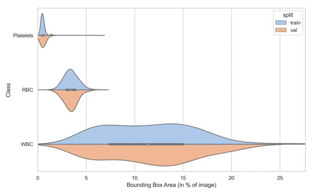
Here we can see that the training and validation sets have similar bounding box area distributions.
Example 2: A Problematic Case
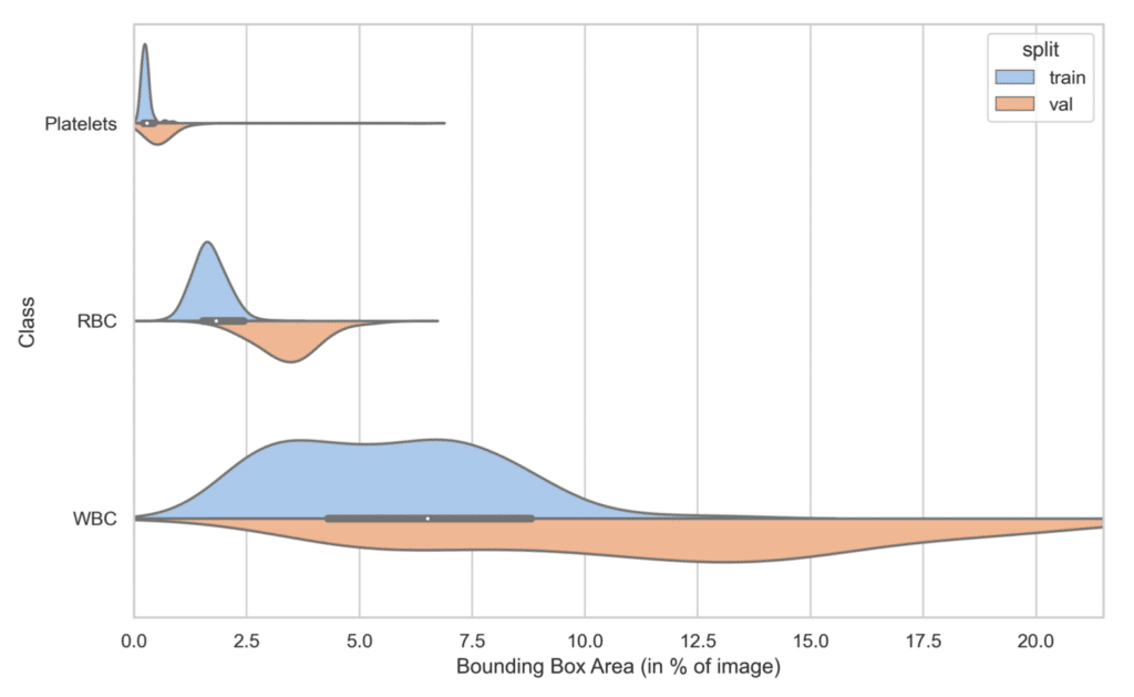
Here, there is a noticeable drift in the distribution between the training and validation sets. This divergence could pose a challenge, as a model trained on this dataset may struggle to accurately detect larger objects in a production environment, owing to inadequate training on such objects.
This discrepancy may suggest that the images in the training set are of a larger spatial scale than those in the validation set. The objects remain the same size as those in the validation set, but the images cover a more expansive area. Consequently, in comparison to the validation set, the objects in the training set occupy a smaller fraction of the total image area.
To address this it could be helpful to randomly crop the training images to achieve a size more consistent with the validation images. Importantly, an exact match in size between the two sets is not necessary. Preserving some degree of variation in resolution can actually serve to enhance the robustness of your model.