
Defining Distribution of Bounding Boxes per Image
Distribution of Bounding Boxes per Image refers to the distribution of the number of bounding boxes appearing in each image in the dataset.
The Importance of the Distribution of Bounding Boxes per Image
Analyzing the distribution of bounding boxes per image holds significant value, particularly when a large number of bounding boxes are observed in each image. This distribution directly reflects the complexity of the images in your dataset; images with more bounding boxes are typically richer in detail and complexity. Consequently, they can be more challenging for models to process accurately, as the model needs to correctly identify and categorize multiple objects within the same frame.
Many object detection models include a parameter to filter the top ‘k’ results. This parameter is essentially a limit on the number of bounding boxes (i.e., detected objects) the model will return after analyzing an image. The rationale behind this is to focus on the most confidently predicted objects, helping to minimize noise and reduce computational demands. However, choosing the right ‘k’ is crucial.
If ‘k’ is too small, the model might overlook some relevant objects. Conversely, if ‘k’ is too large, the model could include many false positives, lowering the overall precision. Understanding the distribution of bounding boxes per image can provide valuable insights to inform this decision.
For instance, if your dataset images typically contain around 20 distinct objects (i.e., have around 20 bounding boxes), setting ‘k’ to 10 might cause the model to miss relevant objects. On the other hand, if most images only contain around 5 distinct objects, setting ‘k’ to 50 could introduce unnecessary computational burden and potential false positives.
In this way, understanding the distribution of bounding boxes per image not only illuminates the intricacy of your dataset but also aids in the calibration of your model parameters, optimizing its performance in detecting and interpreting the objects within your images.
Calculating the Distribution of Bounding Boxes per Image
To calculate the distribution of bounding boxes per image, iterate over all the images in your dataset.
For each image, count the number of bounding boxes. Do this separately for the training and validation sets.
The result is a distribution of the number of bounding boxes per image, allowing you to compare different datasets’ complexity.
Here’s how Distribution of Bounding Boxes per Image is calculated in DataGradients.
Exploring Distribution of Bounding Boxes per Image Through Examples
Let’s consider some examples to see how knowing your dataset’s distribution of bounding boxes per Image can help identify dataset issues.
Example 1: A Favorable Case
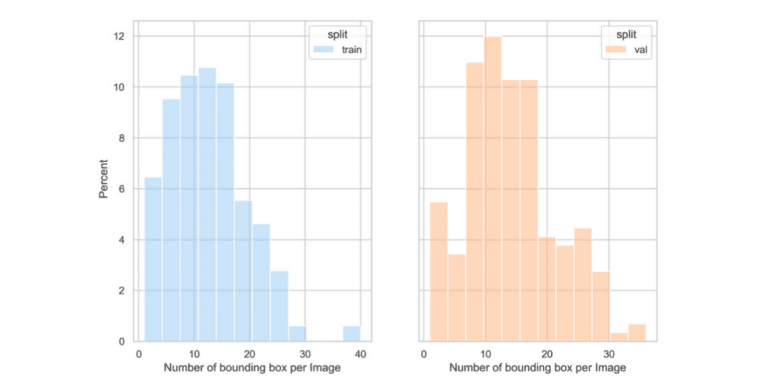
In the above example, the distribution of the number of bounding boxes per image of the training set is similar to that of the validation set.
Example 2: A Problematic Scenario
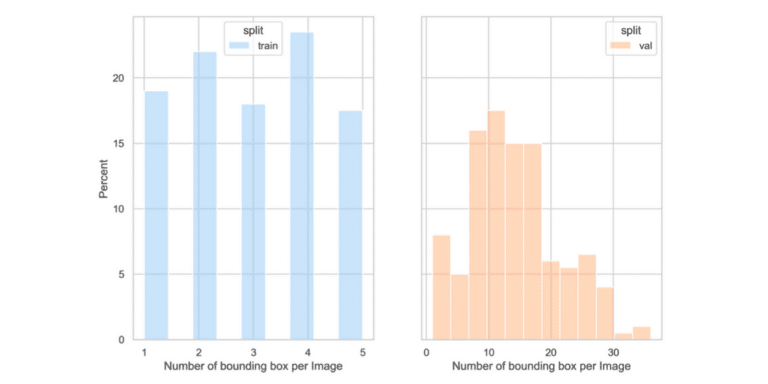
Here, however, the training set has significantly fewer bounding boxes per image.
Uncovering the causes of distribution differences
When a discrepancy appears in the distribution of bounding boxes per image between the training and validation sets, it’s often due to one or more of the following reasons:
Data-related Factors:
- Annotation Inconsistency: Different annotation methods may have been used for the training and validation sets, resulting in inconsistent data.
- Source Diversity: The datasets for training and validation might have been sourced differently, leading to variations in what they represent.
Augmentation-related Factors:
- Excessive Cropping: If areas with a high object density in the training set have been overly cropped, this can skew distribution.
- Over-Downsampling: Downsampling the dataset to an excessively small resolution during training can result in lost or omitted bounding boxes that are smaller than 1 pixel.
Solutions and best practices
To rectify these distribution differences, consider the following strategies:
For annotation inconsistency:
- Set clear annotation guidelines prior to the annotation process and ensure all annotators adhere to them.
- Have each annotator work on both the training and validation sets, rather than assigning separate annotators for each.
For source or subject diversity:
- Apply data shuffling to ensure a more even distribution of images across the training and validation sets, as explained in lesson 1.4.
For augmentation issues:
- Recalculate this feature without resizing to determine if the discrepancy originates from the data itself or the process of downsampling or cropping.
- Avoid downsampling the training set to a resolution so small that bounding boxes are compromised.
- Be mindful of cropping, ensuring important parts of the image aren’t removed.