
Defining Bounding Box Density
Bounding Box Density refers to the spatial distribution of objects of a particular class within images. It is represented as a heatmap, highlighting areas of high density of objects of that class.
Note that common augmentations, such as Mosaic, cropping and padding, can dramatically affect the heatmap; if these are applied to only one of the two sets (training or validation), they are expected to create different heatmaps.
The Importance of Bounding Box Density
By understanding the density of bounding boxes, one can gain insights into the spatial distribution of objects in the dataset.
The heatmap depicts areas of high object density within the images, providing a clear picture of the spatial distribution of objects. Examining the heatmap makes it easy to determine if objects are predominantly concentrated in specific regions or evenly distributed throughout the scene.
This information helps assess whether or not the objects are positioned appropriately within the expected areas of interest.
Understanding your dataset’s Bounding Box Density can also play a significant role in model design. If certain classes within your dataset consistently appear in specific locations, it might suggest that these objects exhibit a location bias within the image. Such objects could potentially benefit from models with larger receptive fields or models that allocate more parameters to their deeper layers. By taking this into account, you can refine your model to better identify and process these specific classes. We discuss this in greater detail in Lesson 5.3.
Calculating Bounding Box Density
To calculate a dataset’s bounding box density, iterate over all the samples in the dataset.
For each sample, scale the bounding boxes to match the shape of the heatmap. Then, for each bounding box, increment the corresponding area of the heatmap.
This gives a heatmap where the value at each point is the number of bounding boxes that cover that point.
Here’s how Bounding Box Density is calculated in DataGradients.
Understanding Bounding Box Density: Examples
To clarify the potential issues related to bounding box density, let’s examine two examples:
Example 1: A Favorable Scenario
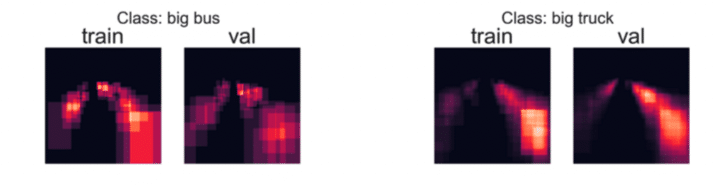
In this instance, we notice similar patterns in the training and validation sets. The spatial distribution of bounding boxes for each class in the training set mirrors that in the validation set. This indicates a well-maintained consistency and can be beneficial for model training.
Example 2: A Potential Issue
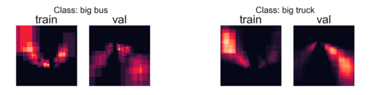
Here, we observe that the placement of objects isn’t consistent. This discrepancy could result from:
- Variations in the data used for the sets,
- Erroneous processing and augmentation transformations.
Although this might not always be problematic (since many computer vision architectures are spatially invariant), it’s essential to investigate the cause. By doing so, you might uncover a fundamental issue with your data or its processing, which could significantly impact your model’s performance.